Finite Element Analysis for Singularly Perturbed Advection-Diffusion Robin Boundary Values Problem ()
1. Introduction
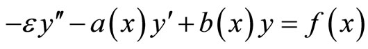
We consider the singularly perturbed advection-diffusion Robin boundary values problem
 (1)
(1)
 (2)
(2)
with sufficiently smooth functions , and a small positive parameter
 . We assume that
  be decreasing monotonously, moreover
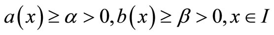 (3)
(3)
which guarantees the unique solvability of the problem. It is well known that there exists a boundary layer of width  at
at  (see [1], K.W. Chang & F.A. Howes 1984). Standard numerical methods for singularly perturbed problem exhibit spurious error unless the layeradapted-mesh, such as Shishkin mesh, B-mesh(see [2-7]) are employed, for the solutions of singularly perturbed problem usually contain layers. The main objective of the paper is to use the method of singular perturbation to give the estimation of error between solution and the finite element approximation w.r.t. some energy norm on shishkin-type mesh.
Throughout the paper, we shall use C to denote a generic positive constant ,that is independent of ε and mesh, while it can value differently at different places, we occasionally use a subscribed one such as C1.
2. Properties of Solution for Continuous Problem
In this section, some properties and bounds of the exact solution and its derivatives are deduced preliminarily.
Lemma 1 (Maximum principle) Let  If
If
 for
for ,
,  ,then
,then
 for
for 
Proof. Assume that there exists  such that
If , then there holds
  which results in a contradiction to
 ;Thus
;Thus .
.
Since we have  the differential operator on
  at
at  gives
gives

which result in a contradiction to  therefore we can conclude that the minimum of
  is non-negative.
Lemma 2 (Comparison principle) If  satisfy
  for
for , and
, and ,
,
 , then
  for all
 .
.
Lemma 3 (Stability result) If , then we have
for all .
.
The Proofs of Lemma 2 and Lemma 3 are followed essentially from Lemma 1. (See [3] Roos, Stynes and Tobiska, (1996)).
Lemma 4 Let  be the solution to (1) (2). then there exists a constant C, such that for all
 , we have the splitting
 (4)
(4)
where the regular component u(x) satisfy
 (5)
(5)
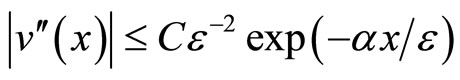
while the layer component  satisfy
 . (6)
. (6)
Proof. It is known that (see [4] Kellogg 1978, Chang & Howes 1984)

We assume  spontaneously since singular perturbation.
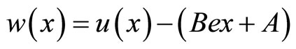
We set  such that
and  on
on  thus
thus  on
on
 and then extended on (0,1) with
 ;
;
Next let
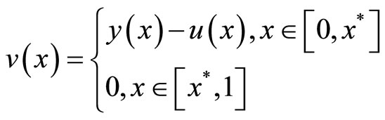
Then considering that  on
on , we know that
  satisfy
 on
on 
3. Simplification
For simplification of the original problem, we set a transformation

then Equation (1), (2) are transformed to


Continuing, we transform the boundary values homogeneously by
at last, the problem (1), (2) are converted to


where in the  posses the same properties as
 , thus we just make discussion on the simplified problem below
 (1’)
(1’)

 (2’)
(2’)
4. The Analysis of Finite Element Approximation
We consider the Galerkin approximation in form of Find  such that
 (7)
(7)
where , the bilinear form

And a natural norm associated with  is chosen by

wherein

is the usual 2-norm.
It is easy to see that  is coercive with respect to
  by the assumption of the monotony of
  which guarantees the existence of the solution of (7) (see [8-10]). Let N be an even positive integer that denotes the number of mesh intervals.
We consider the space of piecewise linear function denoted by  as our work space,
  denotes the piecewise linear interpolant to
  at some special mesh points on I, We’ll utmost estimate the error
 .
.
Firstly we have
 (8)
(8)
For the second term of inequality (8), we make use of the coerciveness, continuousness of  and the Galerkin orthogonality relation:
  to obtain that
Thus
 . (9)
. (9)
Combined with (8), we just need to estimate the interpolation error bound  below.
Lemma 5 The solution  of (1’), (2’) and its piecewise linear interpolant
  satisfy


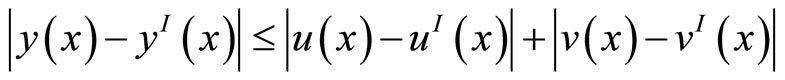
Proof. According to the splitting of , we have correspondingly
From Lemma 1 we have
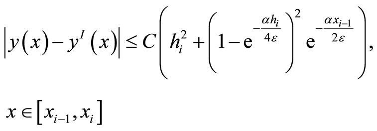
 To obtain the estimation for singular component, we use a Taylor expansion

to express the error bound

Continuously, we use the inequality involved a positive monotonically decreasing function g on 
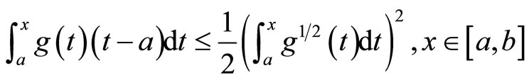
Thus we have

Hence
For the proof of the second statement, we have
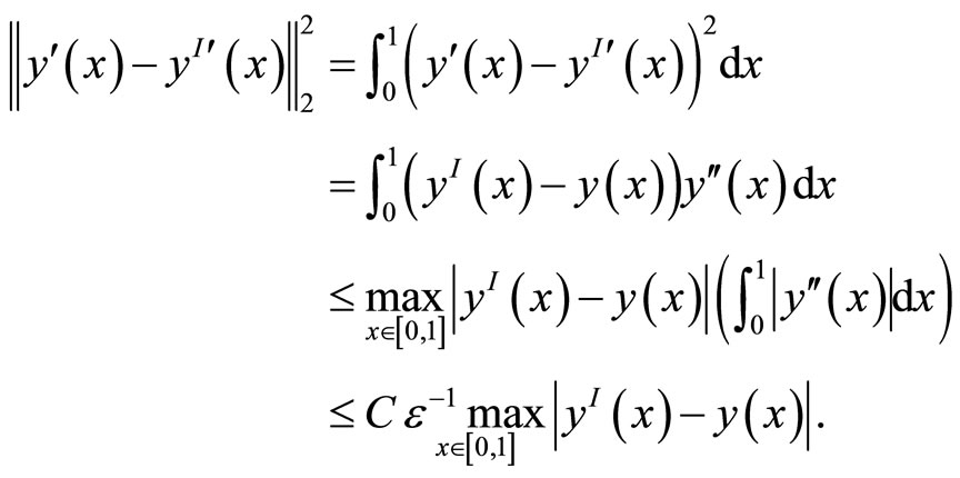
thus, lemma 5 follows.
Theorem For ,
, defined before, when the Shishkin mesh are applied ,we have the parameter uniform error bound in the energy norm naturally associated with the weak formulation of (1’), (2’)
 (10)
(10)
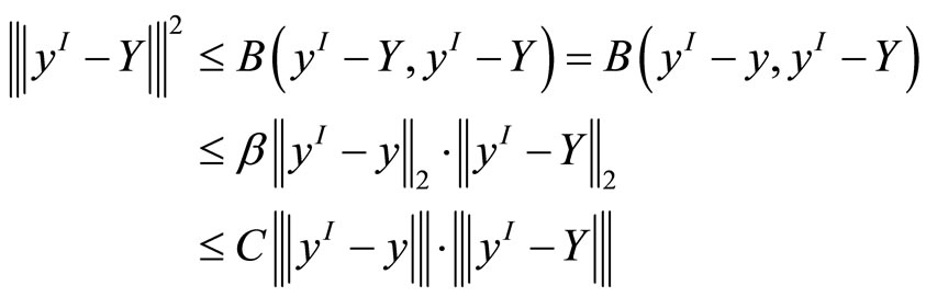
Proof. Firstly, we have by triangle inequality and (9)
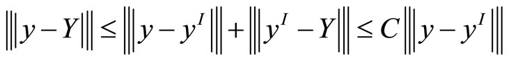

where in C’s and C1 are stated before. thus we have

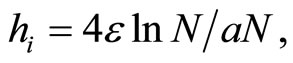
Now we use the classical Shishkin mesh (see [11-13]) by setting the mesh transition parameter defined by
 and allocate uniformly
points in each of  and
and . In practice one typically has
 , we just acquiesce in this case thus
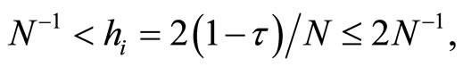
thus for ,
,

Also for 
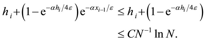
Combining the above two cases reads (10).
Remark. To obtain  estimation, the standard Aubin-Nitche dual verification skill may be involved.
The superconvergence phenomena on Shishkin mesh for the convection-diffusion problems can be discussed according to Z. Zhang (see [13,14]).
NOTES