Variant Map System to Simulate Complex Properties of DNA Interactions Using Binary Sequences ()
1. Introduction
Stream ciphers [1,2] play a key role in modern network security [3,4] especially in multimedia network environments; its core component—pseudo random number generation mechanism [5-7]—takes the central position in modern cryptography [8,9]. Associated with advanced development of bioinformatics, advanced DNA sequencing and analyzing techniques [10,11] have significantly progressed over the past decade.
1.1. DNA Cryptography
DNA cryptography makes joined research in the field of DNA computing and cryptography. Scholars over the world focused on this field and different results are published such as simulating DNA evolution [12], DNA pseudorandom number generator [13-16], DNA cryptography [9,17,18] and so on. However in current situation, DNA cryptography is still at an earlier stage as an emerging area of advanced cryptography.
In typical results of DNA cryptography on encrypttion, different coding schemes could be randomly selected. E.g. the algorithm in paper [17] applies an encoding formula to express the plaintext on DNA sequence: {00→C, 01→T, 10→A, 11→G}; however in paper [18], the same author uses the coding formula {00→A, 01→T, 10→C, 11→G} for the plaintext on DNA sequence. In encryption environment, all 4! = 24 possible encoding methods could be equally used in different applications.
1.2. Stream Cipher HC-256
Stream ciphers are an important class of encryption algorithms. A stream cipher is a symmetric cipher which operates with a time-varying transformation on individual plaintext digits. The ECRYPT Stream Cipher Project (eSTREAM) [1] was a multi-year effort, running from 2004-2008, to promote the design of efficient and compact stream ciphers suitable for widespread adoption. HC-256 is a stream cipher, designed to provide bulk encryption in software at high speeds while permitting strong confidence in its security. A 128-bit variant was submitted in 2004 as an eSTREAM cipher candidate; it has been selected as one of the four final contestants in the software profile [2,4] in 2008 as the most advanced scheme for stream cipher applications in advanced network environment.
1.3. Large Noncoding DNA & RNA
In relation to DNA analysis, visualization methods play a key role in the Human Genome Project (HGP) [19]. After HGP completed successfully, a public research consortium—the Encyclopedia of DNA Elements (ENCODE) was launched by the National Human Genome Research Institute (NHGRI) in 2003 to find all functional elements in the human genome as one of the most critical projects by NHGRI to explore genomes after HGP.
In 2012, ENCODE released a coordinated set of 30 papers published in key Journals of Nature, Genome Biology and Genome Research. These publications show that approximately 20% of noncoding DNA in the human genome is functional while an additional 60% is transcribed with no known function [20]. Much of this functional non-coding DNA is involved in the regulation of the expression of coding genes [21]. Furthermore, the expression of each coding gene is controlled by multiple regulatory sites located both near and distant from the gene. These results demonstrate that gene regulation is far more complex than was previously believed [22]. Mammalian genomes encode thousands of large noncoding RNAs (lncRNAs), many of which regulate gene expression, interact with chromatin regulatory complexes, and are thought to play a role in localizing these complexes to target loci across the genome [23]. Associated with different international projects, larger numbers of Genome Databases are established and mass Genomewide gene expression measurements are developed.
Due to huge amount of DNA sample collections and extremely difficulties to determine their variation properties in wider applications [24-30], it is essential for us to extend advanced DNA analysis models, methods and tools in further extensions to explore emerging models and concepts to interpret complex interactions among complicated sets of DNA sequences in real environments.
1.4. DNA Analysis
DNA analysis plays a key role in modern genomic application [19]. The HGP is heavily relevant to advanced DNA sequencing and analysis techniques. DNA sequences are composed of four Meta symbols on {A, T, G, C} as basic structure. Classical DNA double helix structure makes the first level of pair construction of DNA sequences with A & T and G & C complementary structures as the first level of symmetric relationships. A typical DNA sequencing result is shown in Figure 1(a). Four Meta symbols could be separated as four projective sequences.
In ENCODE, recent Genomic analysis results are indicated that encoded sequences have only 20 percent in human genomes and around 80 percent genomes look like useless sequences. Under further assumptions, it seems that additional symmetric properties are required to satisfy the second, third and higher levels of structural constructions to explore complex interactive properties [24-30].
In current situation, it is necessary for advanced researchers to shift targets in computational cell biology from directly collecting sequential data to making higherlevel interpretation and exploring efficient content-based retrieval mechanism for genomes. Using higher dimensional visualization tools, their complex interactive properties could be organized as different visual maps systematically.
1.5. Variant Construction and DNA
Variant construction is a new structure composed of logic, measurement and visualization models to analyze
 (a)
(a) (b)
(b)
Figure 1. Modern DNA sequencing & their correspondences on variant logic; (a) A sample DNA sequencing and its four projection sequences; (b) Four Meta DNA Symbols and linkages to variant logic.
0 - 1 sequences under variant conditions. The further details of this construction can be checked on variant logic [31,32], 2D maps [33,34], variant pseudo-random number generator [35-37], DNA maps [38] and variant phase spaces [34]. Since the variant system uses another set of four Meta symbols  to describe system, a typical correspondence shown in Figure 1(b) may provide a natural mapping between DNA and variant data sequences.
Since DNA sequences are played an essential role to explore different symmetric properties based on analysis approaches, in this paper, measurement and visual models are proposed systematically to use a fixed segment structure to measure four Meta symbols distributions in their spectrum construction. Under this construction, refined symmetric features can be identified from various polarized distributions and further symmetric properties are visualized.
1.6. Target of This Paper
The target of this paper is to establish the Variant Map System (VMS) as a unified framework to analyze complex DNA interactions on both artificial and natural DNA sequences. The VMS has designed to use variant logic schemes [31-38] applying multiple maps on four Meta symbols as DNA or RNA representations. System architecture of key components and core mechanism on the VMS are described. Key modules, equations and their I/O parameters are discussed. Applying the VM System, two sets of real DNA sequences from both human (noncoding DNA) and corn (coding DNA) genomes are collected in comparison with pseudo DNA sequences generated artificially by HC-256 to show their intrinsic properties in higher levels of similar relationships among DNA sequences on 2D maps. Further descriptions and discussions are provided respectively.
2. System Architecture
In this section, system architecture and their core components are discussed with the use of diagrams. The refined definitions and equations of this system are described in the next section—Variant Map System.
2.1. Architecture
T Architecture he four components of a variant map system are the Binary To DNA (BTD), the Binary Probability Measurement (BPM), the Mapping Position (MP), and the Visual Map (VM) as shown in Figure 2.
The architecture is shown in Figure 2(a) with the key modules of the four core components being shown in Figures 2(b)-(e) respectively.
In the first part of the system, the t-th sequence  on either {0, 1} or {A, G, T, C} are input data to get into the BTD module. The main function of the BTM is to output a unified sequence
  either to transfer a 0 - 1 sequence or to keep a DNA sequence as a pseudo or pure DNA sequence under a set of controlled parameters.
Using this unified DNA sequence, four vectors of probability measurements are created from the t-th selected DNA sequence with  elements as an input. Multiple segments are partitioned by a fixed number of n elements for each segment; at least
  segments can be identified by the BPM component. Next component uses the four vectors of probability measurements and a given k value as input data, a pair of position values are created for each Meta symbol. Four pairs of values are generated by the MP component. Then, in order to process multiple selected DNA sequences, all selected sequences are processed by the VM component and each sequence may provide a set of pair values to generate relevant variant maps to indicate their distribution properties respectively.
With eight parameters in an input group, there are three sets of parameters in the intermediate group and one set of parameters in the output group.
The three groups of parameters are listed as follows.
Input Group:
t An integer indicates the t-th DNA sequence selected, 
 An integer indicates a relationship distance among elements in a binary sequence,
 An integer indicates the mode of elements in a sequence,
  ,
,  for a DNA sequence,
  for a binary sequence
 An integer indicates the number of elements in the t-th DNA sequence,
 An input data vector with
  elements,
 An integer indicates the number of elements in a segment,
V A symbol is selected from four DNA symbols 
 An integer indicates the control parameter for mapping,
Intermediate Group:
 A unified DNA vector with
  elements,
 Four sets of probability measurements with
 Four paired values,
Output Group:
 Four 2D maps,
2.2. BTD Binary to DNA
The BTD component shown in Figure 2(b) is composed of one module: BTD itself. Five parameters are shown as

Figure 2. Variant Map System (VMS) and key components (a) Architecture; (b) BTD component; (c) BPM component; (d) MP component; (e) VM component.
input signals and one unified vector is generated by the BTD component as the output group.
Input Group:
t An integer indicates the t-th DNA sequence selected, 
 An integer indicates a relationship distance among elements in a binary sequence,
  mode An integer indicates the mode of elements in a sequence,
  ,
,  for a DNA sequence, mode = 1 for a binary sequence
 An integer indicates the number of elements in the t-th DNA sequence,
 An input data vector with
  elements,
Output Group:
 A unified data vector with
  elements,
The BTD component uses an input vector on either binary or DNA format as input, under a set of input parameters to process transformation. The output of the BTD component is composed of a unified vector of DNA format in a given condition.
2.3. BPM Binary Probability Measurement
The BPM component shown in Figure 2(c) is composed of two modules: BM Binary Measure and PM Probability Measurement. Three parameters are listed as input signals; four vectors of binary measures are outputted from the BM component as an intermediate group and four sets of probability measurements are outputted as an output group.
Input Group:
 An integer indicates the number of elements in a segment,
V A symbol is selected from four DNA symbols, 
 A DNA vector with
  elements,
Intermediate Group:
 Four 0 - 1 vectors with
  elements,
Output Group:
 Four sets of probability measurements with
The BPM component transforms a selected DNA sequence to generate four 0 - 1 vectors by BM module for the input DNA sequence. Then four probability vectors are generated by the PM module as the output of the BPM under a fixed length of segment condition.
2.4. MP Mapping Position
The MP component shown in Figure 2(d) is composed of three modules: HIS Histogram, NH Normalized Histogram and PP Pair Position. Two parameters are listed as input signals; four histograms and four normalized histograms are generated from the HIS component and the NH component as intermediate groups respectively. Four paired values are generated by the PP component as the output group.
Input Group:
 Four sets of probability measurements with
 An integer indicates the control parameter for mapping,
Intermediate Group:
 Four histograms for relevant probability measurements,
 Four normalized histograms for relevant probability measurements,
Output Group:
 Four paired values,
The MP component uses probability measurements as input, under a given k condition to generate each relevant histogram and its normalized distribution. The output of the MP component is composed of four paired values controlled in a given condition.
2.5. VM Visual Map
The VM component shown in Figure 2(e) is composed of one module: VM Visual Map. Three parameters are input signals. Collected all selected DNA sequences, four 2D maps are generated by the VM component as the output result.
Input Group:
 All DNA sequences are selected,
 An input data vector with
  elements,
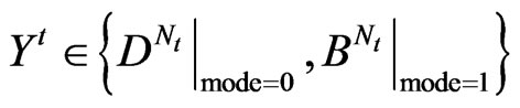
 Four paired values for the t-th DNA sequence,
Output Group:
 Four 2D maps,
The VM component processes all selected DNA sequences as input to generate paired values for each sequence. The output of the VM component is composed of four 2D maps to show the final visual distribution for the system.
3. Variant Map System
3.1. Initial Preparation
Let r an input parameter make all pairs of elements with r distance in a binary sequence to be a pseudo DNA vector, mode a controlled parameter indicate various pairs of operations performed if . Denote
  a binary base and
  a DNA base respectively.
3.2. BTD Module
Let  an input sequence with N elements,
 ,
,
 . This input vector could be expressed as follows.
 ,
,
 . (1)
. (1)
Let X denote a DNA sequence with N elements, D denote a symbol set with four elements i.e. . This type of a DNA sequence can be described by a four valued vector as follows:
 ,
,
 . (2)
. (2)
From this input and associated parameters, following operations are performed.
If , for all
 , the output vector is equal to the input vector.
 (3)
(3)
If , for all pairs of I and
  elements of
  the I-th output element
  can be determined by the corresponding conditions shown in Figure 1(b) as follows.

 (4)
(4)
In both conditions,  will be a unified vector with four values as the output of the BTD shown in Figure 2(b).
e.g. Let a binary sequence , three pseudo DNA sequences
  can be represented as follows.

Selecting a certain  value, a relevant pseudo DNA sequence can be generated from an input binary sequence.
3.3. BM Module
For a given I-th element, four projective operators can be defined and denoted as  .
.
 (5)
(5)
Applying the four operators to all elements, the DNA sequence X can be reorganized into the four binary sequences of 0 - 1 values. i.e.

 (6)
(6)
e.g. let a DNA sequence  , its four binary sequences can be represented as follows.

It is interesting to notice that the basic relationship between a DNA sequence X and its four  sequences are exactly same as in a modern DNA sequencing procedure to separate a selected DNA sequence into the four Meta symbol sequences shown in Figure 1(a). This correspondence could be the key feature to apply the proposed scheme naturally in simulating complex behaviors for any DNA sequence.
The projection  provides the essential operation in the BM component as the first module shown in Figure 2(c).
3.4. PM Module
For this set of the four binary sequences, it is convenient to partition them into m segments and each segment contained a fixed number of n elements.
For the l-th segment, let  , the I-th position will be
 , four probability measurements
  can be defined.
 (7)
(7)
Under this construction, four sets of probability measurements established.
 (8)
(8)
The probability operator  generates four probability measurement vectors in the PM component as the second module shown in Figure 2(c). After the BM and PM processes, the whole procedure of the BPM component is complete in Figure 2(c).
3.5. HIS Module
Since the BPM generates four sets of probability measurement, it is necessary to perform further operations in the MP component shown in Figure 2(d) as follows.
In the HIS component as the first module in Figure 2(d), each probability sequence  can be calculated from n positions, at most n + 1 distinguished values identified in a vector. Under this organization, a histogram distribution can be established.
Let  be a histogram operator, for each position, it satisfies following relation,
 (9)
(9)
Collecting all possible values, a histogram distribution can be established,
 (10)
(10)
The histogram  is the output of the HIS module. Four histograms are generated after HIS process. Further normalized process will be performed in the NH component as the second module in Figure 2(d).
3.6. NH Module
Under this construction, a normalized histogram can be defined as
 (11)
(11)
After the NH component processed, its output provides the PP component for further operations as the third module in Figure 2(d).
3.7. PP Module
Relevant probability vectors have  distinguished values; four sets of normalized vectors can be organized as a linear order as follows,
 (12)
(12)
Under this condition, four linear sets of probability vectors are established,
 (13)
(13)
For four vectors, their components can be normalized respectively,
 (14)
(14)
Four sets of probability vectors are composed of a complete partition on their measurements.
Using this set of measurements, two mapping functions can be established to calculate a pair of values to map analyzed DNA sequence into a 2D map as follows.
Let  and
and  or
or  be a pair of values defined by following equations,

 (15)
(15)
In the PP component, four paired values are generated and each pair indicates a specific position on a 2D map for the selected DNA sequence. The core operations of three key components: BTD, BPM and MP for a selected sequence are performed in Figures 2(b)-(d).
3.8. VM Module
Since only one point of a 2D map is determined for a selected DNA sequence, it is essential to apply relative larger number of DNA sequences as inputs to generate visible distributions. This type of operations will be performed in the VM component shown in Figure 2(e).
In a general condition, the VM component processes a selected data set  composed of T sequences, the t-th sequence with
  elements can be expressed by

Each sequence can be processed to apply the same procedures of the BTD, BPM and MP components. Since for each segment, its length n will be fixed for all selected sequences, it is essential to make number of segments be  in convention to match each sequence. Under this expression, the last module VM collects all T pairs of positions on relevant 2D visual maps as follows,
 (16)
(16)
A sample 2D map of VM is shown in Figure 3; this provides an assistant illustration for this type of visual maps on a case of multiple sequences.
Under this construction, a total number of T DNA sequences are transformed as T visual points on four 2D visual maps that would be help analyzers to explore their intrinsic symmetry properties among four binary sequences.
4. Sample Results on 2D Maps
Two types of data sets are selected for comparison. The first type of data sets is real DNA data sequence collected from both human and plan genomes to illustrate their differences on 2D maps. The second type of data set is collected from the Stream Cipher HC-256 to generate a pseudo random binary sequence under a certain condition.
4.1. DNA Data Resources
It is important to use some real DNA sequences to illustrate various test results of the VMS. Two sets of DNA sequences are selected and relevant resource features are described as follows.
The first data set originally comes from the human genome assembly version 37 and was taken from the reference sequences of 13 anonymous volunteers from Buffalo, New York. Hi-C technology used to analyze chromatin interaction role in genome. From a genomic analysis viewpoint, this set of data may contain more complex secondary or higher level structures. A special structure nearly the GRCh37 DNA sequence has been identified to explore their spatial characteristics. After positive and negative sequencing, each data file contain 2700 DNA sequences and each sequence has around 500 elements stored in two files left and right respectively.
The second DNA data set are selected from some plant gene database for comparison. One set of DNA sequences of Corn genomes are stored in file 201-500 that contains 2700 DNA sequences and each sequence has around 200 - 600 elements. It may be ordinary single sequences without complex secondary structures.
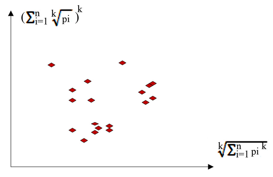
Figure 3. A sample 2D map of VM on multiple sequences.
4.2. Pseudo DNA Data Resources
The Stream Cipher HC-256 has being used to generate a binary sequence on a total length of 2700 × 500 bits in the file hc256 that has been partitioned as 2700 subsequences and each sub-sequence in 500 bits.
Using the VMS in various parameters, three sets of pseudo DNA sequences are generated and their 2D maps are illustrated, analyzed and compared in following subsections.
4.3. Sample Results
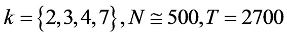
Using the three files of DNA sequences and one pseudo binary sequence in three parameters, six sets of 2D maps are listed in Figures 4-9 under different conditions to illustrate their spatial distributions using the VMS in a controllable environment.
In Figure 4, three groups of eighteen 2D maps are shown in the range of 

 for comparison; (a1)-(a6) six
 maps for the file Right; (b1)-(b6) six
  maps for the file 201-500; (c1)-(c6) six
  maps for the file hc256 respectively.
In Figure 5, four groups of sixteen 2D maps for the file right are listed in the range of 
 ; (a) group (a1)-(a4) four
  maps; (b) group (b1)-(b4) four
  maps; (c) group (c1)-(c4) four
  maps; (d) group (d1)-(d4) four
  maps.
maps.
In Figure 6, four groups of sixteen 2D maps for the file hc256 are listed in the range of ,
, ; (a) group (a1)-(a4) four
  maps; (b) group (b1)-(b4) four
  maps; (c) group (c1)-(c4) four
  maps; (d) group (d1)-(d4) four
  maps.
maps.
In Figure 7, four groups of sixteen 2D maps for the file right are selected in the range of 
 ; (a) group (a1)-(a4) four
  maps; (b) group (b1)-(b4) four
  maps; (c) group (c1)-(c4) four
  maps; (d) group (d1)-(d4) four
  maps.
maps.
In Figure 8, three groups of twelve 2D maps for the file hc256 are compared in the range of .
.  (a) group (a1)-(a4) four
  maps
maps ; (b) group (b1)-(b4) four
  maps
maps ; (c) group (c1)-(c4) four
 maps
maps .
.
In Figure 9, three groups of twelve 2D maps for two files right and hc256 are compared in the range of ; (a) the file right n=15, mode=0; (b) the file hc256 n = 12, mode = 1, r = 1; (c) the file hc256 n = 12, mode = 1, r = 3; (a1)-(c1)
  maps; (a2)-(c2)
  maps; (a3)-(c3)
  maps; (a4)-(c4)
  maps.
maps.
4.4. Result Analysis of 2D Maps
Six groups of 2D maps contain different information, it is necessary to make a brief discussion on their important issues as follows.
The first group of results shown in Figure 4 presents
three sets of eighteen 2D maps from three data files: right, 201-500 and hc256 undertaken various lengths of basic segment from 3-50 to illustrate their variations respectively. Six 2D maps of each group in Figure 4 (a1)-(a6) show significant trace on their visual distributions; the numbers of main visible clusters identified are decreased when the length of segment has being increased e.g. (a3)-(a6). However lesser length of segment does not provide refined visual distinctions with larger region in fuzzy areas e.g. (a1) and (a2). From a structural viewpoint, middle ranged numbers of length provide better clustering results e.g. (a3)-(a5) for further analysis targets. To check another six 2D maps of Figure 4 (b1)-(b6) for the file 201-500, significantly different visual distributions can be observed than (a1)-(a6); the numbers of main visible clusters identified are decreased when the length of segment has being increased less significantly e.g. (b4)-(b6). However lesser length of segment does not provide refined visual distinctions with wider regions in fuzzy areas e.g. (b1)-(b3). In generalmiddle ranged numbers of length still provide better clustering effects e.g. (b4)-(b6) for further analysis purpose. To check six 2D maps of Figure 4 (c1)-(c6) for the file hc256 r = 1, similar visual distributions can be observed than (a1)-(a6) and significantly differences are observed than (b1)-(b6); the numbers of main visible clusters identified are decreased when the length of segment has being increased less significantly e.g. (c3)-(c6). However lesser length of segment does provide refined visual distinctions with regions in fuzzy areas e.g. (b1). In general, middle ranged numbers of length still provide better clustering effects e.g. (c2)-(c4) for further analysis purpose. From their distributions, groups (a) and (c) have shared much stronger similar properties than group (b).
It is interesting to observe different maps when control parameter k changed. Four groups of sixteen 2D maps for the file right are shown in Figure 5 on the range of ; four groups in (a)-(d) provide four maps to share the same other parameters with different k values. Checking visible clus-


Figure 9. Three groups of twelve maps in the ranges: N = 500, T = 2700, k = 7; (a) Real DNA data; (a1)-(a4) DNA sequences from the file right; (b)-(c) Simulation Data; (b1)-(b4) Binary Sequences from the file hc256, r = 1; (c1)-(c4) Binary sequences from the file hc256, r = 3. (a1)-(a4) Four maps for the file right, n = 15, mode = 0; (b1)-(b4) Four maps for the file hc256, n = 12, r = 1, mode = 1; (c1)-(c4) Four maps for the file hc256, n = 12, r = 3, mode = 1.
ters in different maps, it is important to notice nearly same numbers of clusters identified in the same group, but different groups may contain significantly different numbers. Lesser k value (e.g. k = 2) makes a tighter distribution and larger k value (e.g. k = 7) takes better separation on the maps. Through k = 7 maps provide better separation effects, it is easy to observe their y axis values already in 108 range.
Four groups of sixteen 2D maps for the file hc256 are shown in Figure 6 in the range of 
 . This group of 2D maps can be compared with 2D maps in Figure 5. Under the same parameters, similar visible effects and feature clustering properties could be observed if various k values are selected.
Using a set of selected parameters, two groups of eight 2D maps are compared in Figure 7 for two files: left, right to explore higher levels of symmetric properties for secondary or higher levels of structures potentially contained in DNA sequences. Selected parameters are in the range of . Group (a) provides four
  maps (a1)-(a4) for the file left; group (b) uses four
  maps (b1)-(b4) for the file right.
In convenient description, let ~ be a similar operator, for groups (a) & (b), four pairs of {(a1)~(b1), (a2)~(b2), (a3)~(b3), (a4)~(b4)} maps i.e. (left-A ~ right-A, left-T ~ right-T, left-G ~ right-G, left-C ~ right-C) have a stronger similar distribution between left & right. In addition, only two clustering classes could be significantly identified as {(a1)~(a2)~(b1)~(b2), (a3)~(a4)~(b3)~(b4)} i.e. (left-A ~ right-A ~ left-T ~ right-T, left-G ~ right-G ~ left-C ~ right-C) respectively. This type of similar clustering distributions may strongly indicate eight maps with intrinsically higher levels of DNA sequences with extra A-T & G-C pairs of symmetric relationships between two files: left & right.
Using a set of selected parameters, three groups of twelve 2D maps are listed in Figure 8 for the file hc256, r = {1, 2, 3} to explore properties for their higher levels of structures potentially contained in pseudo DNA sequences. Selected parameters are in the range of . Group (a) provides four
  maps (a1)-(a4) for r = 1; group (b) uses four
  maps (b1)-(b4) for r = 2 (c) uses four
  maps (c1)-(c4) for r = 3. Using a similar operator, for groups (a)-(c), four pairs of {(a1)~(b1)~(c1), (a2)~(b2)~ (c2), (a3)~(b3)~(c3), (a4)~(b4)~(c4)} maps i.e. (A(r = 1)~A(r = 2)~A(r = 3), ···, C(r = 1)~C(r = 2)~C(r = 3)) have a stronger similar distribution among r = {1, 2, 3}. In addition, only two clustering classes could be significantly identified as {(a1)~(a2)~(b1)~(b2)~(c1)~(c2), (a3)~ (a4)~(b3)~(b4)~(c3)~(c4)} i.e. three maps are shown in (A~T, G~C) respectively.
In a convenient comparison, using a set of selected parameters, three groups of twelve 2D maps are compared in Figure 9 for the files: right and hc256, r = {1, 3} to check their distribution properties contained in both DNA and created pseudo DNA sequences. Group (a) provides four  maps (a1)-(a4) for the file right; groups (b) and (c) provide four
  maps (b1)-(b4) for hc256, r = 1 (c) and (c1)-(c4) for hc256, r = 3.
Using a weak similar operator ;, for groups (a)-(c), four pairs of {(a1);(b1)~(c1), (a2);(b2)~(c2), (a3)~ (b3)~(c3), (a4)~(b4)~(c4)} maps have a stronger similar distribution between r = {1,3} and a weak similar distribution on A & T cases. In addition, only two clustering classes could be significantly identified as {(a1)~(a2); (b1)~(b2)~(c1)~(c2), (a3)~(a4)~(b3)~(b4)~(c3)~(c4)} i.e. three maps are strongly shown in relationships among (A~|;T, G~C) for different cases respectively.
In addition, this set of results illustrates directly visual comparisons with stronger similarity between DNA and pseudo DNA on VMS maps, their similarly clustering distributions may indicate those maps with comparable mechanism to express real DNA sequences with extra A-T & G-C pairs of symmetric relationships in their higher levels of relationships applying the Stream Cipher mechanism.
5. Conclusions
This paper proposes architecture to support the Variant Map System. Using a binary random sequence as input, a set of special pseudo DNA sequences can be generated. Under variant measures, probability measurement and normalized histogram, a pair of values can be determined by a series of controlled parameters. Collecting relevant pairs on multiple DNA sequences, four 2D maps can be generated.
The main results of this paper provide the VMS architecture description in diagrams, main components, modules, expressions and important equations for the VMS. Core models and diagrams, sample results are illustrated to apply two types of data sets selected from real DNA sequences and generated from the pseudo random sequences from the Stream Cipher HC-256 for comparison under the VMS testing. After proper set of parameters selected, suitable visual distributions could be observed using the VMS. Results in Figures 4-9 provide useful evidences systematically to support proposed VMS useful in checking higher levels of symmetric/similar properties among complex DNA sequences in both natural and artificial environment.
This construction could provide useful insights to spatial information on complex DNA expressions especially on large encoding RNA/DNA construction via 2D maps to explore higher levels of complex interactive environments in near future.
6. Acknowledgements
Thanks to the school of software Yunnan University, to the key laboratory of Yunnan software engineering and the key laboratory for Conservation and Utilization of Bio-resource for excellent working environment, to the Yunnan Advanced Overseas Scholar Project (W8110305), the Key R&D project of Yunnan Higher Education Bureau (K1059178) and National Science Foundation of China (61362014) for financial supports to this project.
NOTES
#Corresponding author.