Optimal Investment and Proportional Reinsurance with Risk Constraint ()
1. Introduction
Maximizing the expected utility of wealth is an important objective for an insurer. To achieve this goal, there has been much attention in the literature in security market and/or reinsurance-related products [1-9]. The insurer is tempted to put his/her surplus into the risky investment so as to obtain a higher potential return. However, maximizing profit should not be the only objective. As risky investment could result in a heavy loss, a shrewd insurer should strike a balance between the amount of risky assets and risk-free assets, such that they are kept within bounds. In today’s challenging economic climate, it is clear from the latest report, entitled Financial Reform: A Framework for “Financial Stability” released by The Group of Thirty (G30), that firms must balance risk with caution between the long-term interests of shareholders and returns to shareholders.
One instrument of risk control is reinsurance, which transfers part of the risk exposure to another insurer. In this way, the utility is improved because the reinsurance will help absorb the possible major loss resulting from an insurance claim. However, reinsurance is costly since the insurer has to pay hefty premiums to the reinsurer. This will, in turn, reduce the utility significantly. Thus the optimal choice of reinsurance is also an important issue for the insurer. With a certain risk measure in place, we can control the exposure to risky assets and determine the level of necessary reinsurance.
In risk management, a popular risk measure is valueat-risk (VaR). VaR has emerged as an important risk management tool to estimate the potential loss over a given time period with a given probability. With VaR as the risk constraint, Kostadinova [2] studied the problem of maximizing the expected utility of wealth. In [2], the optimal investment strategy is sought by maximizing the expected wealth of the insurance company with the value-at-risk constraint imposed at the initial date. However, VaR of the portfolio is never reevaluated after the initial date. This is different from the practice adopted by most financial institutions where they use VaR for internal risk control, and VaR is reevaluated frequently. Because the VaR of the portfolio after the initial date, the probability of portfolio losses below the prescribed maximum VaR can become zero after the initial date and yet the trader is still allowed to continue to follow the original trading strategy. This trading strategy is clearly inconsistent with the purpose of imposing the VaR constraint.
In this paper, by allowing both the opportunities of investment and proportional reinsurance, we consider the problem of maximizing the expected exponential utility for the final wealth subject to the VaR constraint. Here, the utility reflects the amount of satisfaction gained by the financial agent from wealth. We impose the VaR as a risk constraint at each instant and emphasize the need for the repeated recalculation of VaR in practice. Moreover, the constraints are calculated abstracting from withininterval trading, based on the available information. In this way, it can be assured that the constraint is consistent with the strategy, see [10-14].
In solving this optimal investment and proportional reinsurance problem, one popular way is to employ the stochastic dynamic programming approach [1,9,15,16]. By using the dynamic programming principle, the problem is reduced to solving a Hamilton-Jacobi-Bellman (HJB) equation, which is a second order linear partial differential equation. A key assumption in this approach is that the value function of the problem is a  function. This assumption is needed to ensure to obtain the existence of a classical solution to the problem. However, the HJB equation is highly nonlinear. Even its numerical solution is difficult to obtain. This is especially true when the risk constraint is taken into account simultaneously. Moreover, the dynamic programming approach deals with the problems in Markov model setting. For the Martingale approach, it works well in a complete market. Since every Martingale relative to a Brownian filtration can be represented as a stochastic integral with respect to the underlying Brownian motion, the integrand in this representation can lead to the portfolio that we are seeking. However, in an incomplete1 market with a constraint on the strategy or when the number or the risky asset is smaller than the dimension of the driving Brownian, this line of arguments fails.
In this paper, we study an investment reinsurance problem with a dynamic risk constraint. The approach that we will propose is much easier than the traditional one. It transforms the stochastic optimal control problem into a deterministic optimal control problem. Although the parameters for the assets are assumed to be deterministic functions of time, it appears possible to be extendable to cases, where the parameters are measurable with respect to some filtration defined in the work. Our approach is applicable to cases with or without constraints on the strategy, and whether or not the model setting is Markovian. This provides a different perspective to the investigation of the investment reinsurance problem in actuarial science.
The rest of the paper is structured as follows. In Section 2, we present the investment-reinsurance model with dynamic risk constraint. Here, we consider the wealth maximization problem with the exponential utility function, which plays a prominent role in insurance mathematics and actuarial practice. The exponential utility function is the only utility function under which the principle of “zero utility” gives a fair premium that is independent of the level of reserve of an insurance company (see Gerber [17], page 68). In Section 3, by decomposition, we show that this constrained stochastic optimal control problem can be simplified significantly, reducing to a constrained deterministic optimal control problem and then to a finite-dimensional optimization problem, which can be tackled by classical computation techniques, such as [18-20]. In Section 4, we demonstrate the effectiveness of this method through carrying out numerical experiments for cases of complete and incomplete markets, where the risky assets are fewer than the uncertainty factors (i.e., the dimension of the Brownian motion). We also conduct numerical experiments to investigate the effect of the VaR constraint on the strategy.
2. The Model and the Problem
Suppose that the accumulated claim process  of an insurer can be modeled as:
 (1)
(1)
where  is a standard Brownian motion defined on a complete probability space
 . Let
. Let  be the filtration generated by
 . The surplus process
 , which represents the liquid assets of the company (also called the risk or the surplus process) is taken as the state variable. With a safety loading
 , the continuously paid premium is assumed to be
 . In the absence of control, the surplus is governed by
 (2)
(2)
where  denotes the initial reserve.
The proportional reinsurance  is a predictable process with
 , for
, for . If the risk exposure of the company is fixed, then the reinsurer pays
  of each claim while the rest is paid by the insurer. To this end, the cedent diverts part of the premiums to the reinsurer at the rate of
  with a proportional loading of
 .
.
Suppose that the insurer is also allowed to invest its surplus. Assume that the market consists of a risk-free asset and  risky assets. The dynamics of the risk-free and the risky assets evolve according to
 (3)
(3)
and
 (4)
(4)
respectively. Here, the vector
is a  -dimensional standard Brownian motion independent of
  on a probability space
 . We use superscript “
 ” to denote the transpose of a vector or matrix throughout this paper. The vector
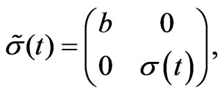
is the appreciation rate, the matrix  is the
volatility with
 ,
,
and
 .
.
Assume that ,
,  and
and  are deterministic functions of t. Let
  denote the natural filtration generated by
 .
.
Let
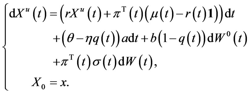
represent the amount invested in the risky asset at time . When both optimal investment and proportional reinsurance are included in our problem formulation, incorporating the strategy
in (2), the dynamics of the resulting wealth process  follows
We denote
 .
.
Set
 with
with
 .
.
The strategy
(equivalently, ),
),
 is said to be
  if 1) it is
  -progressively measurable2)
 -almost surely3)
 .
.
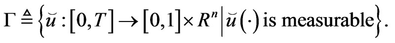
Let  be the class of all such
  strategies. We assume that the following assumption is satisfied.
Assumption 2.1. There exist constants  and
and  such that
 (5)
(5)
where
 .
.
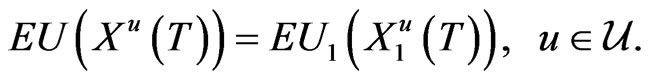
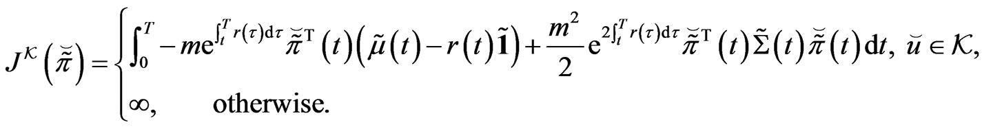
Problem ( ). Given the wealth process (5), find an admissible strategy
  such that the expectation of the final wealth utility defined by
 (6)
(6)
is maximized, where the constant  is the risk aversion parameter (see Pratt [21]).
Now we specify the dynamic risk and impose it as the risk constraint for the optimal investment and reinsurance problem. Suppose that the portfolio is adjusted frequently over time so that the interval from time  to time
  is small, where
 . Here,
  is the risk evaluation horizon, or the risk horizon for short. We consider the loss from time
  to
to . Denote
and
 .
.
Suppose that
is unchanged in the interval , i.e.,
 .
.
We have

It follows that
 (7)
(7)
where
 (8)
(8)
Then, the mean and variance of  are, respectively, given by
 (9)
(9)
and
 (10)
(10)
Let  denote the discounted loss
 .
.
It follows from (10) and (9) that
 (11)
(11)
Let the maximal risk be less than or equal to , i.e.,
 (12)
(12)
Then, the portfolio constraint is
 (13)
(13)
With , namely,
  , the constraint (13) defines a convex set. In this work, we assume that
 .
.
3. Deterministic Reduction
When the market is  in the sense that
  and no constraint is imposed on the strategy, Bai and Guo [15] investigate the problem with short-selling constraint. However, when the strategy is constrained in a general closed convex set due to the presence of the dynamic risk constraint, it is not known if there exists a smooth solution to the associated HJB equation or not. In fact, even if we could show the existence of a smooth solution, this second order nonlinear PDE is difficult to solve, even numerically.
For the stochastic optimal control problem considered in this paper, since the utility function is an exponential function. We will show that it can be reduced to a deterministic optimal control problem via a suitable decomposition. It is further reduced, by the control parametrization technique [22], to a deterministic finite-dimensional problem. A numerical solution of this deterministic optimization problem can be obtained using existing optimization software packages, such as NLPQLP ([18-20]).
We first present a transformation theorem that links the original stochastic optimal control problem with the deterministic optimal control problem. Before stating the theorem, we need to introduce the following notations. For any path , denote
 . Let
. Let
Theorem 3.1 Suppose that
where  is deterministic for all
 , and
, and  is a
is a  martingale. Then,
 (14)
(14)
Furthermore, denote
and let
If , then
 (15)
(15)
Proof. From the properties of Martingale, we have
As
 it follows that (14) holds.
From the notation of , we see that, as
 ,
,
 (16)
(16)
and
 (17)
(17)
It follows from (16) and (17) that
This, together with (14), implies the validity of (15).
This theorem shows that if the decomposition holds, the optimal strategy is the same for all paths, because the parameters ,
,  and
and  are deterministic.
Remark 3.1 Suppose that the parameters ,
, and
and  are
are  -progressive measurable. Since
 the stochastic optimal control problem is reduced to the deterministic optimal control problem with every path.
3.1. The Equivalent Problem
In this subsection, we will show that our problem satisfies the decomposition assumption specified in Theorem 3.1.
Rewrite the dynamics (5) as:
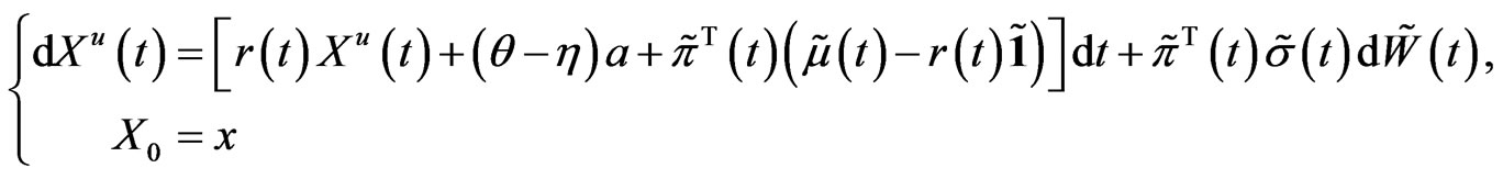
where
 (18)
(18)
Applying Itô’s differentiation rule to (18), we obtain
 (19)
(19)
Thus,
 (20)
(20)
Denoting , we have
 (21)
(21)
and
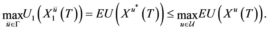
Obviously,  is a Martingale under Assumption 2.1. By Theorem 3.1, the original problem can be reduced to the deterministic optimal control problem
 (22)
(22)
Notice that (22) is also equivalent to the following problem.
Problem ( ). Find
  such that
 (23)
(23)
is minimized, subject to
 (24)
(24)
In the next section, we will show that Problem  admits an optimal solution.
3.2. Existence of Optimal Solutions
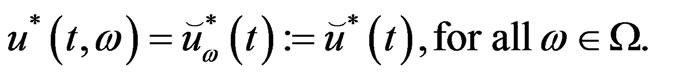
From Theorem 3.1, we see that the optimal strategy is the same for almost all the sample paths. Thus, it suffices to seek a deterministic control strategy for Problem  if all the required assumptions are satisfied.
Let  denote the class of all
  functions.
If , define
For Problem , it is easily seen that if
 , we have that
 , and then
 . Thus, we can consider the following Problem
  with a smaller control set
 , instead of Problem
  with
with .
.
Note that  is a Hilbert space equipped with the inner product of
  and
and  defined by
 (25)
(25)
Let . Then, we have the following result.
Theorem 3.2 Consider Problem , where the function
  is defined by
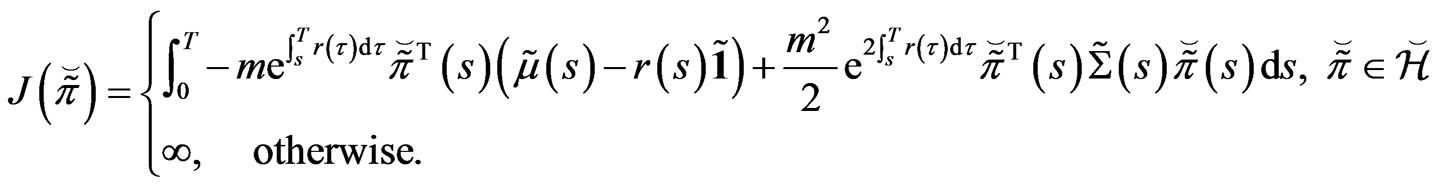
Then, the following properties are satisfied.
1)  is convex;
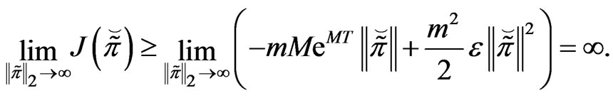
2)  is coercive, i.e.,
and
3)  is lower-semicontinuous, i.e.,
 (26)
(26)
for every  and
and , with
4) There exists a  such that
 .
.
Proof. 1) The convexity is obvious, since
and
are concave.
1) From Assumption 2.1, we obtain
 (27)
(27)
3)
 (28)
(28)
Also,
 (29)
(29)
Thus, 3) holds.
4) From Ekeland and Temam [23], a
a  such that
 .
.
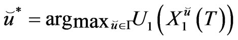
Proposition 3.1 The optimal strategy
is given by
with  being its value function.
Proof. From the expression of , it is easily seen that the pointwise optimal strategy is just the optimal strategy at time
 . The result in Bai and Guo [15] is a special case with constant parameters.
Using an argument similar to that given for Theorem 3.1, we can concentrate on finding a deterministic strategy from
 .
.
Corollary 3.1 Define
Then, there exists a  such that
 .
.
Proof. The proof is similar to that given for the proof of Theorem 3.1 and hence is omitted here.
Let the strategy in Proposition 3.1 be constrained to lie in a closed convex set . Then, the following result holds.
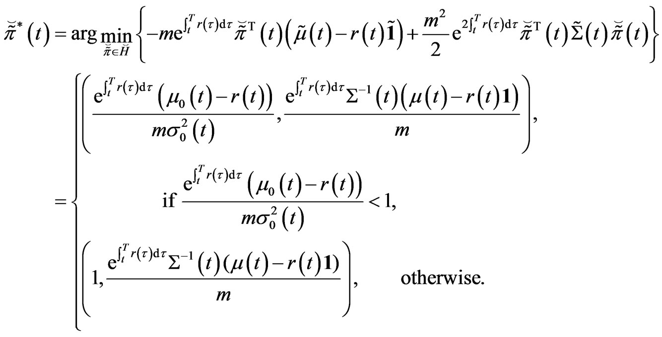
Proposition 3.2 The optimal strategy is given by
 (30)
(30)
with  being its value function.
Although it is difficult to obtain an explicit solution to (30), we can solve this finite-dimensional optimization problem numerically. This is much simpler than dynamic programming, which involves solving a second order nonlinear PDE with constraint. It is also much simpler than the Martingale approach for which it is required to consider the replicate portfolio with constraint.
4. Numerical Experiments
We will develop a numerical method for constructing an approximation of  and then calculating
 . In solving the deterministic constrained optimization problem, we use the control parametrization method (see [18-20]). Let the time horizon
  be partitioned into
  subintervals, and let
  be approximated as a piecewise constant function, given by
 (31)
(31)
where  and
and  is the indicator function defined by
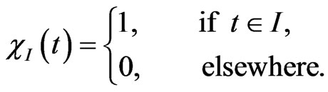
For each ,
,  is a vector specifying the value of
  on the sub-interval
 . Such a strategy should be chosen such that (23) is minimized subject to the dynamics (24). Then, Problem
  can be solved as an optimization problem, and various optimization software packages, such as NLPQLP (see [18-20]), can be used for this purpose.
Consider a complete market where the number  of stocks is equal to the dimension of the driving geometric Brownian motion. The proportional reinsurance
  is the only constraint. In this market, Proposition 3.1 has given the explicit expression of
  and
and . Here, two sets of parameters are used to show that when the trading interval approaches to zero the solutions converge to those in [15].
Case I ( when the reinsurance constraint is inactive). The model parameters are:

and . Figures 1 and 2 plot the risky investment and the proportional reinsurance, respectively.
Case II ( when the reinsurance constraint is active).
 .
.
the proportional reinsurance  for cases with or without risk constraint. In Figure 3, the risky investment under the risk control is compared with the risky investment without control.
To show the effectiveness of the method, we also solve the problem under this assumption . Here, we assume that there is one risky asset, and the Brownian Motion is two-dimensional. The following parameters are used:

Figures 4 and 5 plot the risky investment and the proportional reinsurance, respectively.
In this example, parameters are assumed to be constants, taking the values:
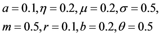
and . Figure
  compares the risky investment
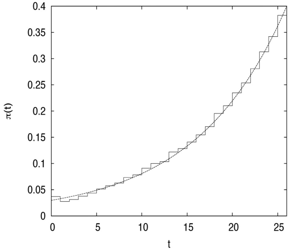
Figure 1. The risky investment in case 1.
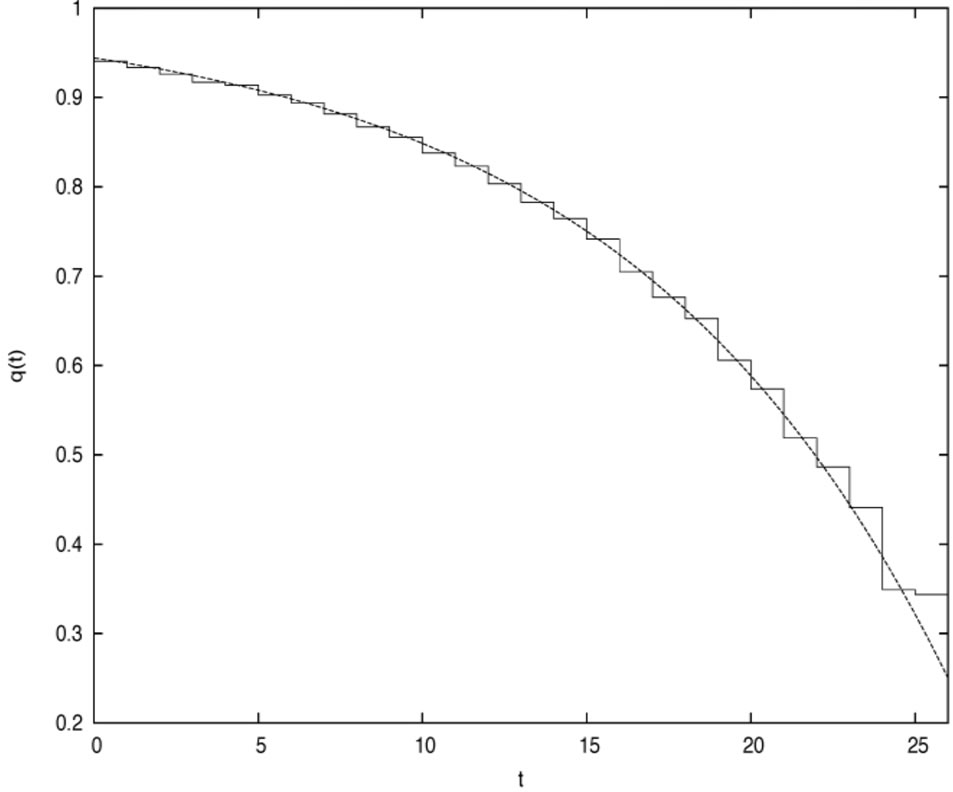
Figure 2. The proportional reinsurance in case 1.
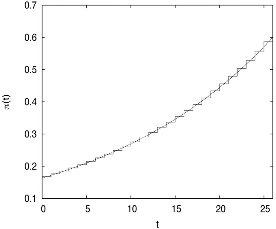
Figure 3.The risky investment in case 2.
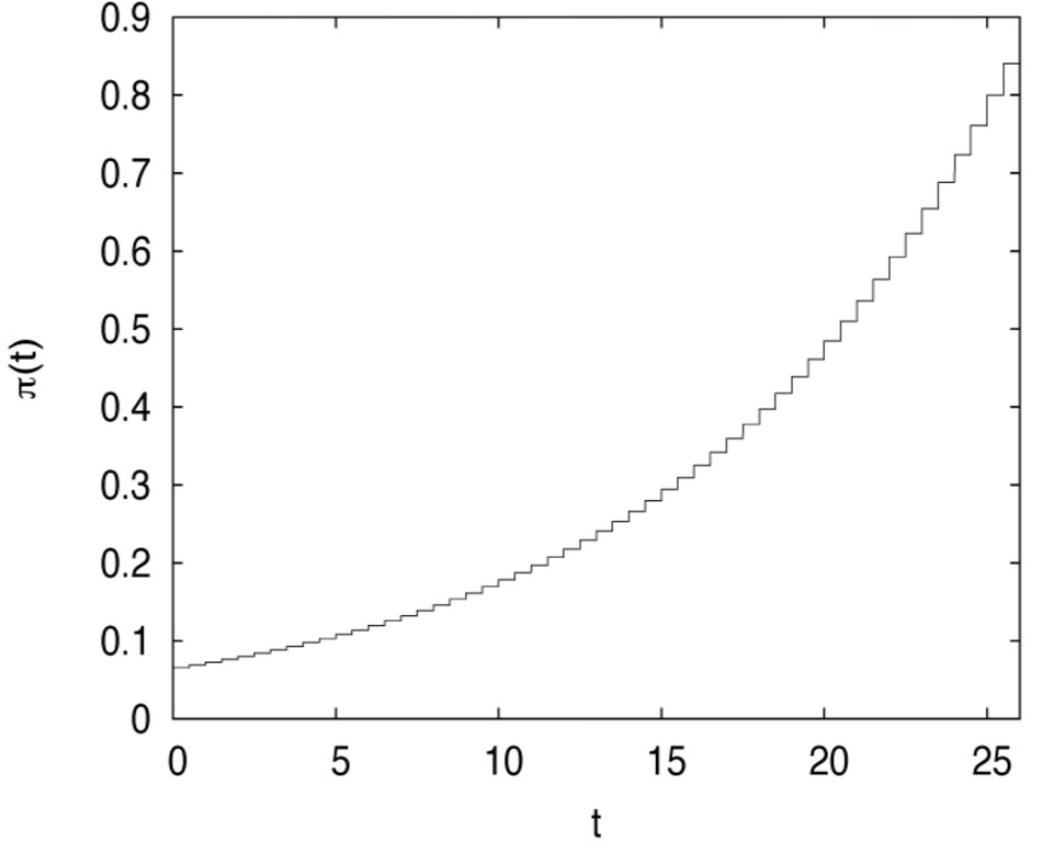
Figure 4. The optimal risky investment in the incomplete market (n < m).
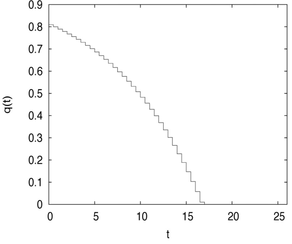
Figure 5. The optimal proportional reinsurance in the incomplete market (n < m).
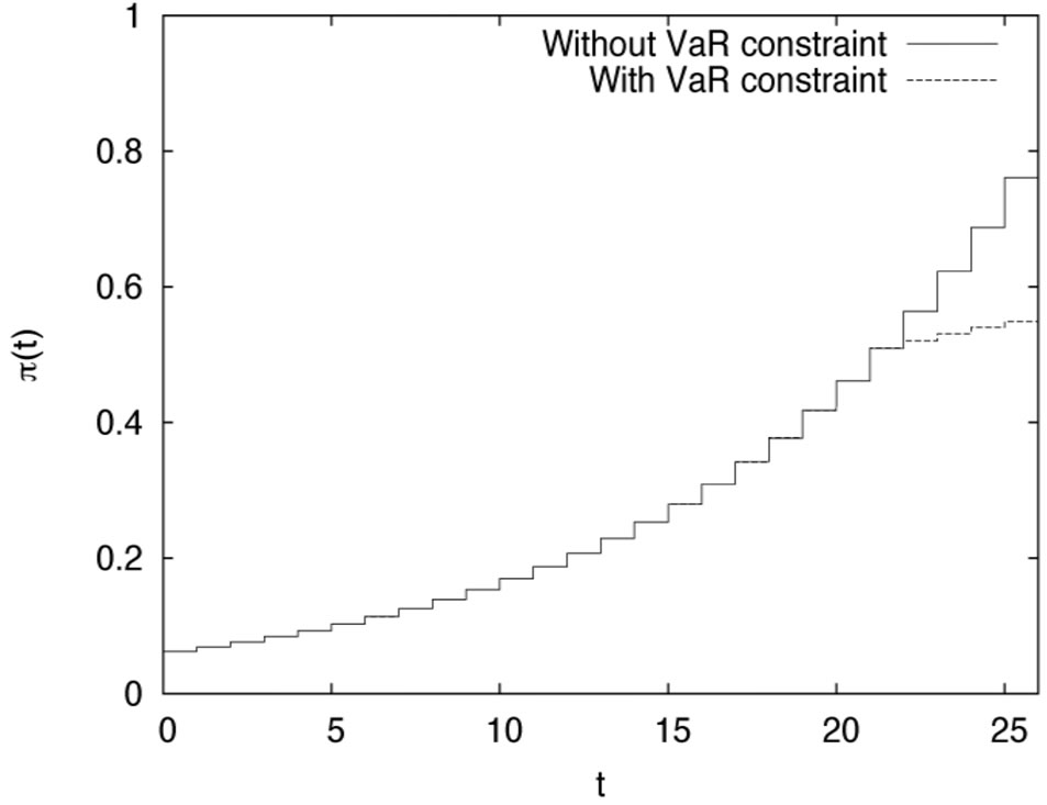
Figure 6. The risky investment compared in the cases: with and without constraint.
in the constrained case with the risky investment without VaR constraint. It is easily seen from Figure 6 that if VaR is active, the risky investment should be cut down consistent with the purpose of the risk management. Figure 7 plots the proportional reinsurance, also for both cases. If the constraint is active, the proportional reinsurance should be increased, when compared with the case of no constraint. We can show its validity under the assumption that  is increasing with
 . To be more specific, let the optimal strategy for the case without constraint and that with constraint be denoted by
  and
and , respectively. Then,
 ,
, .
.
In fact, to satisfy the constraint, we require that either
 or
or .
.
without loss of generality, assume that . If
. If
 then it is clear that the result holds. Otherwise,
 which means that
  is in the constraint set. However,
 which is a contradiction to the fact that
  is optimal. Thus, it follows that
 ,
, 
if  is increasing with
 . In fact, this condition is reasonable as the time horizon
  is small. From Figure 8, we see that VaR is stabilized once the risk constraint is active.
5. Conclusion
In this work, we considered the optimal investment and proportional reinsurance problem with VaR as the dynamic risk constraint. By employing a decomposition approach, we transformed the stochastic optimal control problem into an equivalent deterministic optimal control problem. This equivalent problem is solvable by existing optimal control techniques. It is observed that when the risk constraint is active, the insurer should decrease the investment on risky asset, while increasing the proportional reinsurance. This is consistent with the risk management. The method proposed in this paper is effective for the case with or without constraint. It is also effective in complete and incomplete market(i.e., the number of risky assets is fewer than the dimension of uncertainty). Our approach appears possible for extension to the case when the parameters are  -progressively measurable.
6. Acknowledgements
The first author and second author gratefully ac
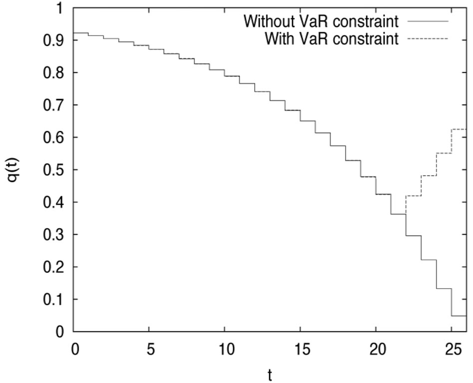
Figure 7. The proportional reinsurance compared in the cases: with and without constraint.
knowledge the financial support from the Research Grants Council of HKSAR (CityU 500111). The first author is thankful for the support of Natural and the Science National Foundation of China (11301559).
NOTES