Bioinformatic Game Theory and Its Application to Biological Affinity Networks ()
1. Introduction
Phylogenetic methods are used to reconstruct the evolutionary history of amino acid and nucleotide sequences. The number and diversity of tools for phylogenetic analysis are continually increasing. Classic phylogenetic methods assume that evolution is a tree-like (bifurcating) branching process, where genetic information arises through the divergence and vertical transmission of existing genes, from parent to offspring. However, when there are reticulate evolutionary events, such as lateral gene transfer (LGT) or hybridization of species, the evolutionary process is no longer tree-like. Such evolutionary histories are more accurately represented by networks [1-3]. The purpose of this paper is to illustrate a game theoretic formulation of evolution which allows us to simultaneously construct an affinity network and a profile for each of the taxa in the network.
The development of analytical tools to generate network topologies that accurately describe evolutionary history is an open field of research. Early network construction methods often employed some appropriate notion of distance between taxa. Posada and Crandall [4] explain why networks are appropriate representations for several different types of reticulate evolution and describe and compare available methods and software for network estimation. One of the earliest methods for phylogenetic network construction was the statistical geometry method [5]. The authors in [6] use a least-squares fitting technique to infer a reticulated network. Other network construction methods can be found in [2,7-9], each of which is useful in modeling a particular kind of data.
Differentiating between vertical and lateral phylogenetic signals is a challenging task in developing accurate models for reticulate evolution. In order to establish a definition for vertical versus lateral transfer it must be that some component of evolutionary signal recovered from a set of genes be awarded privileged status [10]. In the genomic context, vertical signals are assumed to reside within a core set of genes, shared between genomes. The best examples of such sets are the 16S and 18S ribosomal DNA sequences, often used to infer organismal phylogeny [11].
When conflicting phylogenetic signals are combined, relationships amongst taxa that appear to be vertical may in fact be lateral and vice versa, resulting in a set of invalid evolutionary connections [10]. This phenomena is observed, for example, in the thermophilic bacterium Aquifex aeolicus, which has been described as an early branching bacterium with similarities to thermophiles [12] or a Proteobacterium with strong LGT connections to thermophiles [13].
A comprehensive map of genetic similarities which encapsulates the results of all phylogenetic signals is a desirable goal. Lima-Mendez et al. [14] developed a methodological framework for representing the relationships across a bacteriophage population as a weighted edge network graph, where the edges represent the phagephage similarities in terms of their gene content. The genes within the phage were assigned to modules, groups of proteins that share a common function. The authors used graph theory techniques to cluster the phage in the network, and then analyzed the ‘module profile’ for each of the clusters in order to identify modules that were common to phage within the clusters.
Holloway and Beiko [10] introduced the framework for an evolutionary network known as an intergenomic affinity graph (IAG). An IAG is a directed, weighted edge graph, where each node represents an individual genome and an edge between two nodes denotes the relative affinity of the genetic material in the source genome to the target genome. The assignment of edge weights in the IAG is based on the solutions to a set of linear programming (LP) problems. A noteworthy feature of the IAG is that the LP derivation of the edge weights does not force the relationship between two genomes to be symmetric.
Here we introduce a novel game-theoretic formulation for evolutionary analysis. In this context we use the term evolution as a broad descriptor for the entire set of mechanisms driving the inherited characteristics of a population. The key assumption in our development is that evolution (or some subset of the mechanisms therein) tries to accommodate the competing forces of selection, of which conservation force (e.g. functional constrains) seeks to pass on successful structures and functions from one generation to the next, while diversity force seeks to maintain variations that provide sources of novel structures and functions. In other words, we assume that evolution seeks to maximize these two competing objectives. This hypothesis is naturally modeled through the use of game theory, which is suitable for optimizing competing goals in various applied fields. We will further restrict our game model to a zero-sum game because the zerosum hypothesis closely mirrors one of the fundamental principles in nature—the conservation of mass and energy. That is, an atom, nucleotide, or amino acid used up for conservation will not be available for diversification. From a population genetics view, this can be understood as new mutations will be ultimately either lost or fixed. Also, the zero-sum assumption can also be justified as the first order approximation of all competing objectives in games. As a result, our formulation leads to the simultaneous construction of an affinity network and a profile for each of the taxa in the network.
The paper is organized as follows: Section 2 contains a discussion of definitions and notation for a biological affinity network, as well as the development of our game theory model. Also in Section 2 we describe the construction of the affinity network graph as well as the profiles for each of the network taxa, and apply our technique to a multidomain protein family. We summarize our bioinformatic game theory in Section 3. Lastly, all important and pertinent results and proofs about twoplayer zero-sum games are reviewed and compiled in the Appendix.
2. Results and Discussion
We begin this section by defining a biological affinity graph for a given set of taxa. Next, we establish the game-theoretic approach to evolution and demonstrate how this can be used to formulate an LP problem for a given reference taxa in the set, whose solution yields the set of evolutionary neighbors for the reference taxa with respect to all the taxa in the network.
2.1. Biological Affinity Graphs
A taxon space is defined by a set of biological entities, each of which is in turn defined by a set of components. For example, if the entities in the taxon space are defined to be genomes the components will be genes, while if proteins are the taxa the components will be functional or structural domains. Given the taxon space and the corresponding component space we will construct an affinity network (Figure 1(a)).
We use the affinity graph definition similar to that of [10]. A biological affinity graph,  , for a given set of taxa is a directed graph such that each vertex in the set
  uniquely corresponds to one taxon, and all edges have nonzero weights with the incoming edges to any given vertex summing to 1. (The distinction between whether the edges are incoming or outgoing is determined by the construction of the similarity matrix, to be discussed in more detail later.) An example of such a network can be seen in Figure 1(b). An edge from vertex
  to
to  is present if and only if the edge weight
  is strictly positive. The edge weight
  is a measure for the affinity of member
  to
to  relative to all other members of
 . No edge is drawn from any node to itself (i.e.,
 ) by convention.
The network graph is constructed in a taxon-by-taxon approach. For each member of the taxon space we construct a similarity matrix. In these matrices, we compare the amino acid (or nucleotide) sequences of each component as a first order approximation. Suppose there are a total of  components,
  , found in the
  members of
 . Then, as exhibited in Figure 2,
 (a)
(a) (b)
(b)
Figure 1. (a) Protein/domain space and protein networks. Each protein is composed of a set of domains (shown in the domain space), and groups of proteins from the protein space form protein families (i.e. protein clusters). Within each protein family there exists a network graph. In this diagram the individual proteins are represented by a linear string of domains and their network edges are exhibited with dashed lines; (b) Method overview. It shows the pipeline for constructing a protein affinity network from a set of domain architectures.
the similarity matrix,  , of a given reference member
  is an
is an  matrix, where
  is the similarity score of component
  in member
  to member
 . This entry may be considered as a proxy for the mutual information between
  and
and  with respect to component
  in that the higher the value the more similar the pair are in component
 . The values in the reference column (the
  column) will not be used in calculation and therefore we arbitrarily set
  for all
 .
.
As mentioned above, the edge directionality of our network graph depends on the construction of the similarity matrix. If the scores are established using the reference taxon,  , as the intended parent sequence, the edges with nonzero weights will be the outgoing edges of the corresponding node, representing a likely ancestordescendent directionality. Similarly, if the scores are constructed to permit the inference that the reference taxon is a descendent sequence, the edges with nonzero weights will be the incoming edges to the reference node. If there is no obvious parent-offspring directionality, as is the case in the similarity matrix construction for our analysis, either convention may be used but only to keep track of the model solutions.
Once the edge weights are found for all , they in turn, as mentioned above, define the network matrix
  as shown in Figure 2. The directed network graph is then constructed according to the weight matrix
  and vice versa. Furthermore if the matrix is block diagonalizable as explained in Figure 2, then each (irreducible) block defines a distinct subnetwork graph, referred to as a cluster. Therefore, the construction of any directed affinity network graph is reduced to finding the weight vector
  n.
n.
2.2. Evolution as a Game
Our idea for the construction of the edge weights  is based on the assumption that evolution seeks to maximize both conservation and diversity. First we will view the interwoven relationships of taxa as the result of all evolutionary processes by, to name a few, mutation, recombination and gene transfers (both vertical and lateral), all taking place amongst thousands of individual organisms contemporaneously in space and repeated for thousands of generations, and all driven by some particular selective forces. Second we will view that the net effect of these processes as a non-cooperative, twoplayer game in which one player, or one force, is to maximize the genetic conservation, or self-preservation, so that deleterious changes are eliminated and successful (or non-deleterious) structures and functions are passed on from one generation to the next; and the other player, or the other force, is to maintain the genetic diversity and to maximize evolutionary resources where novel structures and functions can be tried out. We will assume, for this paper and for the purpose of being a primary approximation, that the two goals are polar opposite because conservation as characterized by structural and functional similarity is negatively correlated with diversity which is characterized by the reverse. This first order approximation can also be justified by the principle of mass and energy conservation in nature. That is, genetic materials and natural resources that are devoted for conservation will not be available for divergence (or in population genetics, extinction vs. fixation). In short we will view evolution as a repeatedly played game with the aim to maximize both preservation and divergence simultaneously. We suppose that the net effect of playing this game of evolution is the closeness, or the distance, of one member to other members in the taxon space, and this effect is to be captured by the frequencies, explained below, with which a reference taxon has interacted with the other taxa.
The goal of our game-theoretic model for evolution is to find a Nash equilibrium [15-17] of the expected payoff for similarity,  , by determining the affinity probability vector
  to maximize
  while simultaneously minimizing it (i.e., maximizing the diversity) by finding the novelty probability vector
  . The conservation-diversification dichotomy interpretation for the y and x probability vectors can be explained as follows. In the case of a pure “diversity” or “component” strategy being played, say
 ,
,  for
for  and
and , that is, when component
  of the reference member
  is used to measure divergence it is the taxon (or taxa)
  having the largest similarity score
  that should be picked as the countering “conservation” or “taxon” strategy to maximize the similarity score
 . Here
  denotes the subset of the
  components that are present in the reference taxon
 . Thus
  for these
 , and the
  sum to 1. This gives the conservation interpretation of the y solutions.
On the other hand, in the case of a pure ‘conservation’ or ‘taxon’ strategy being played, say ,
,  for
for  and
and , that is, when
  is used to measure affinity to the reference
  it is those component(s) having the smallest similarity score
  that stands out and should be picked as the countering “diversification”, or “component” strategy to minimize the similarity score
 . That is, these
  are positive and sum to 1, and permit the interpretation for divergence.
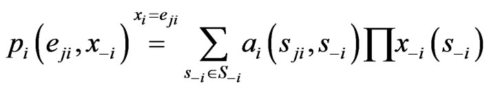
As we mentioned before, since all evolutionary processes—all kinds of genetic transfers or otherwise—take place amongst all organisms all the time, the evolutionary state we observe today would be the result of the frequencies with which all pure conservation strategies and all pure diversity strategies are played one event a time, and by our proposed game-theoretical model these frequencies are approximated by the solution y and x to the following min-max problem (see Equation (1)).
The solution to this problem exists and is exactly a Nash equilibrium point (see Appendix). The optimal expected similarity score,  , is the so-called game value.
There are two different ways to find a Nash equilibria (NE) for two-player zero-sum games. One is through a dynamical play of the game to find an NE asymptotically which is modeled by the Brown-von-Neumann-Nash (BNN) system of differential equations. The other is by the simplex method in linear programming. The Appendix gives a comprehensive compilation for all fundamental results of both methods.
Here we present a mechanistic derivation of Nash’s map. Nash used this map to prove the existence of NE for all non-cooperative games (Appendix). Our derivation is extremely relevant to our game theory formulation for bioinformatics. It gives a plausible answer to the question how an NE is realized by nature. It shows that evolution or individual organisms need only be driven by their immediate, short term gain in game play payoff to reach a globally attractive Nash equilibrium. Here is an outline of the scenario, which works for not only two but for any number of player types of a game or multiple competing objectives of a process.
In the case that a game is played by large populations of all types repeatedly for a long time so that the time between consecutive plays can be blurred to view the game as played continuously and the play strategy frequency for player type- ,
,  , changes continuously, where
  is the mixed strategy probability or frequency vector,
 . Each
  corresponds to the
  th strategy of the type-
 players, and
  can be interpreted to be the fraction of the player type-
 (1)
(1)
population that uses its pure strategy . Consider it at time
  and a
and a  time later,
 . We would like to understand how
  changes from
 . We will do so probabilistically.
Let  be the scalar inertia probability by which an individual of the type-
 population plays the same strategy with probability
  at time
  as at time
 . Then,
  is the non-inertia or kinetic probability with which an individual of the type-
 population chooses or adapts to a particular strategy, including the choice of playing the same strategy at time
  as at time
  because it is advantageous to do so, or because the individual organism is driven to do so due to selection. Let
  be the conditional play probability vector given that the play is kinetic,
  , then by elementary probability rules
 (2)
(2)
The scalar marginal probability  and the conditional probability vector
  are derived as follows. First we assume the advantage for type-
 player’s kinetic strategy switch or adaptation depends on its total (scalar) excess payoff
  from the current play frequency (Appendix, also [16,17]), where
  denotes the current play frequency for all player types with probability vector
  for player type-
 . That is, if
 , then all plays are of the inertia kind,
  , and
, and  without adaptation. Next, for the
  case, we assume the
  th kinetic frequency is
  , where
  (Appendix) is the
  th strategy’s excess payoff from the current play for the player type-
 ,
, . That is, the strategy switch to strategy
  for the type-
 players is strictly proportional to its excess payoff against the total
 . As for the scalar marginal inertial probability
 , we assume it is a function of the total excess payoff as well as the time increment
 . Specifically, consider the probability equivalently in its reciprocal
 , which represents all fractional possible choices for each inertia choice. The fractional possible choices automatically include the inertia choice itself so that
  always holds. Then at
 , we must have this trivial boundary condition
 , the default inertia choice only for lack of time to adapt. Assume the fractional possible choices increase linearly for small time increment
 , we have
  where 1 represents the inertia choice itself and
  represents the rate of increase in the kinetic choices, which may include the choice of maintaining the same strategy play, because of its excess payoff is positive, and all other kinetic strategy adaptations. We assume the rate of the kinetic choice change is proportional to the total excess payoff,
  , i.e., the greater the excess payoff the more play switches in the population for a greater payoff gain. As a result,
  and equivalently,
 . With the functional forms for
  and
and  above, we have
 (3)
(3)
which is exactly the Nash map ([17]) if  and
and . From Equation (3) we also have

and hence the following equivalent system of differential equations
 (4)
(4)
after a time scaling by . This type of equations was first introduced in [18] by Brown and von Neumann to compute an NE for symmetrical zero-sum games and the derivation of Equation (4) from the Nash map
 was first noted in [19].
However, our derivation of the Nash map from the time evolution relationship (2) between inertia and kinetic strategy plays is new to the best of our knowledge. The derivation immediately suggests an evolutionary mechanism as to how a Nash equilibrium point may be realized or reached because the process or the game play is driven by the excess payoff at every step of the way, which can be interpreted as a mechanism for adaptation and a force of selection. In fact, let

define the total excess payoff potential, then for any two-player zero-sum game Theorem 2 of Appendix shows that  always decreases
  if
if  and
and  for every solution
  of the BNN Equation (4). An NE is reached when there is no more excess payoff left,
 . It shows that as a global dissipative system, any mixed play frequency trajectory will always find a Nash equilibrium by following the down gradient of the excess potential function
 . That is, in their search of greater excess payoffs, the total excess payoff for the players can never increase along any time evolution of their game plays. A computational implication of this theorem is that a Nash equilibrium of any two-player zero-sum game can always be found by the iterates of the Nash map or the solution to the BNN equations for any initial strategy frequency. This result solves the important problem as to how dynamical plays of a zero-sum game driven by individual players seeking out only localized advantages can eventually and collectively find a globally stable Nash equilibrium. Figure 3 shows, for a prototypical two-player zero-sum game, the trajectories of the Nash map for a small time increment
  and the BNN equation converge to an NE which is a saddle point on the payoff surface of one player and a global minimum on the excess potential surface, which can be viewed as a energy function for the dynamics of the BNN equation.
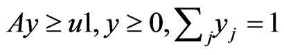
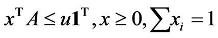
With the existence problem and the search problem for NE solved, we can employ alternative and practical methods to find them. One standard procedure to solve the min-max problem (1) is to solve the following linear programming problem as reviewed in Appendix (see Equation (5)).
There are both commercially available and free packages to solve such LP problems. It is well-known that the y solution and the optimal value  for the objective function
  to the LP problem (5) are exactly the y solution and respectively the game value to the min-max problem (1), and the shadow price or the set of Lagrange multipliers for the LP problem is exactly the x solution to the min-max problem.
2.3. Affinity Network and Component Profile Construction
To complete the outline of our method, the edge weight  from
from  to
to  is assigned to be
  from a Nash equilibrium of the min-max problem for node
 . That is, the y solution, which obviously depends on
  but the dependence is suppressed for simplicity, for each node
  gives the
  th row of the network matrix W of Figure 2. The x solution vector for each
 , is used to define the component profile for the node
 .
.
Thus, by our game theoretic approach the edge weights of the affinity network and its corresponding component profiles are the result of both conservation and diversity being maximized. More specifically, a high edge weight in the affinity graph indicates a strong affinity between taxon pairs relative to the others, and a high row weight,  of node
 , indicates that the reference individual,
  , is somewhat unique or dissimilar with respect to the component
  compared to the other members of the taxon space.
The game values also yield important information about the affinity network. For example, for two topologically identical clusters, it is their average game values that set them apart, which in this sense the cluster with the higher average game value is a “tighter” or a more similar subnetwork than the latter.
The importance of a Nash equilibrium lies in the property that if we change the affinity frequency vector y from its optimal, then we may find a different diversity frequency vector x so that the corresponding expected similarity score is lower than the game value. Similarly, if we change the diversity frequency vector x from its optimal, we may then find a different affinity vector y so that the corresponding expected similarity score is larger. That is, deviating from the conservation optimal distribution may give rise to a greater diversification, and deviating from the diversity optimal distribution may give rise to a greater conservation. The dynamical state of the evolution, according to our model, is literally sitting at a saddle point of the expected similarity function; and the game value is a balanced tradeoff between reproducibility and diversity, a minimally guaranteed affinity.
2.4. An Application to a Multidomain Protein Family
A protein domain is a part of a protein sequence, a structural unit, that can function and evolve almost independently of the rest of the protein. Proteins often include multiple domains. Domain shuffling [20] or domain accretion [21] is an important mechanism in protein evolution underlying the evolution of complex functions and life forms. Figure 4 is a simple example of evolution of multidomain proteins illustrating how multidomain proteins can be evolved from simple single-domain proteins. Multiple evolutionary events including duplication, loss, recombination, and divergence generate complex proteins [22,23]. As shown in Figure 4, the evolutionary process of multidomain protein families also contains network relationships. As a consequence of their com-
 (5)
(5)
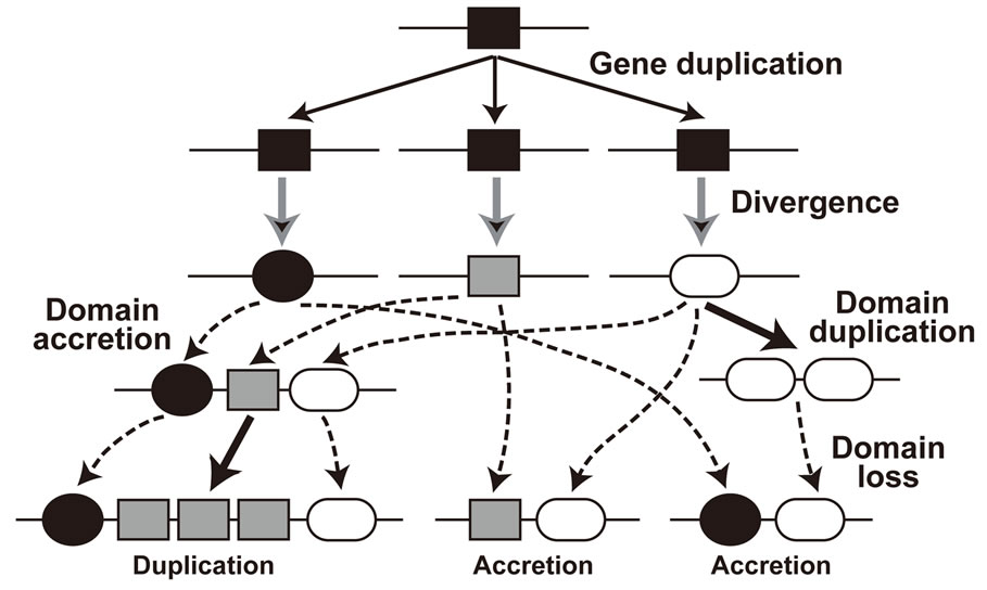
Figure 4. Evolution of multidomain proteins.
plex evolutionary history, a large variation exists in the numbers, types, combinations, and orders of domains among member proteins from the same family.
In order to understand relationships of proteins and their functions, it is important to incorporate domain information when we study multidomain proteins. To show how we can apply our game-theory based method to reconstruct protein networks, we studied an example of the Regulator of G-protein Signaling (RGS) protein family.
We extracted a set of 66 (RGS family protein) sequences from the mouse genome. RGS sequences were found by performing a profile hidden Markov model search in HMMER [24,25] using the Pfam [26] families PF00615 (RGS) and PF09128 (RGS-like) as query sequences and with E-value threshold 10.
This RGS sequence set was subsequently used to HMMER search against Pfam database to find other domains present in the sequences. This step tries to identify all other domains that coexist with the RGS and RGSlike domains in our RGS proteins. From the sixty six RGS proteins, fifty eight Pfam domains (including RGS and RGS-like) were identified. Next, each of the individual domain sequences from each of the RGS proteins was extracted and used as the query sequence in a blastp sequence similarity search [27] against each and every sequence in the RGS protein sequence set.
The BLAST E-value was used as distance measure between each domain and each of the RGS protein sequences, so that an E-value of 0 is expected when using the domain from a sequence to BLAST search against the sequence itself and large E-values are expected when highly diverged domain sequences are identified. If a domain is not found on some sequence, we use 2870 as the maximum distance since on average this is the maximum possible E-value using BLAST on our data search space. In the end, we obtained all the distances between every domain sequence of every RGS protein and every RGS protein sequence. For the entries in each similarity matrix we used a log-transformed score of the E-value with  following [10], where
  is the E-value obtained for the domain query
  against the subject protein
 . With one similarity matrix as the input, the LP problem shown in (5) can be solved. The solutions to the set of LP problems provide the edge weights for the RGS protein affinity network.
In the resulting network, eight clusters were identified within this protein space. Clusters are labeled according to their average game values, in descending order. The first four clusters are exhibited in Figure 5. As mentioned before, the game values yield important information about the clusters present in the affinity network. For example, Cluster 1 and Cluster 4 each include three proteins (nodes) and are topologically identical. However, their average game values are 146.5601 and 68.3844, respectively, which in this sense Cluster 1 is a tighter or a more similar subnetwork than Cluster 4.
The domain profile across the proteins in the first four clusters in the RGS affinity network is exhibited in Figure 6. The proteins are grouped by the clusters in the network graph. Clear profile pattern differences exist between the model clusters. For many of the clusters, the proteins contain the same domain and the weights placed on these domains in the LP solution (the  vector) for each of the proteins are similar. The profile also highlights domains that are unique to specific clusters. For example, in the set of clusters shown the Pfam domain PF00631.17 is hallmark to Cluster 4 because it is present in all members of Cluster 4 and not elsewhere.
For a regular phylogenetic analysis of multidomain proteins, usually only sequence information of domains shared across all member proteins (e.g., RGS domain) can be used. A phylogenetic analysis using RGS domain sequences showed phylogenetic clusters largely consistent with the network clusters our method identified (data

Figure 5. RGS protein affinity network. This protein network is a subset of the larger RGS sequence set (see Figure 1 for information). RGS proteins contain various domains in different combinations, but all share the RGS domain (Pfam family: PF00615 or PF09128). We identified in total 58 Pfam domains on the 66 RGS proteins. In this graph, the nodes represent distinct proteins, and the edges are directed so that the incoming edge weights of each node sum to 1. The edge color indicates the edge weight, with darker (black) edges indicating high weights and lighter (red) edges indicating low weights. Clusters in the network, represented by different node colors, are labeled in descending order according to their average game value, i.e., Cluster 1 denotes the cluster with the largest average game value. See Figure 6 for the domain profiles for the proteins.
not shown). However a regular phylogenetic analysis cannot represent information from many other domains that are not shared, nor network relationships as our affinity networks reveal.
As an additional validation of the network clusters, we provide the information for the proteins within each cluster in Figure 7. It clearly shows that different domain architectures are represented in different clusters. Sequence divergence within the same domain type (e.g., RGS_RZ-like domain for RGS 19/20 vs. RGS 17 proteins) is also recognized in separating Clusters 1 and 2. Furthermore we note that isoforms (proteins coded in alternatively spliced transcripts derived from the same gene) of the same gene fall into the same cluster even if some domains are missing in different isoforms as shown in the beta-adrenergic receptor kinase 2 isoforms 1 and 2 in Cluster 3. Therefore, using our game-theoretic framework, we incorporated both sequence diversity and domain information and produced a valid RGS protein network.
3. Concluding Remarks
Using game theory to study biological problems was introduced by Maynard Smith [29,30]. Our formulation of evolution as a game is different from his evolutionarily stable strategy theory (ESS) for animal behavior and conflict. In ESS, there are the literal players in individual animals and the literal strategies that the players use in competition for reproduction and ecological resources. In our formulation however, evolution as a process is modeled as a game in which, the player (or the numerous players) is the selective force which operates everywhere, any time, in every biological process. Whenever an evolutionary event consists of an exact vertical transmission of a piece of genetic information, evolution plays the role of conservation, and otherwise it plays the role of diversification. That is, conservation and diversification are the two inseparable sides of evolution. The strategies of evolution as a process are its products. At the genome level, any enhancement of affinity between two genomes is the play of conservation whereas any widening of difference in a gene or gene composition between the genomes is the play of diversification. In fact, the genome network constructed in [10] can now be exactly replicated by our game theoretical approach. At the protein level, the overall similarity between two proteins is of the conservation play and any diverging domain difference is of the diversity play. In each level, the payoff of the game or process is not literal but the evolutionary similarity or dissimilarity in their bioinformatics broadly construed, which can be measured in terms of various informational distances.
Our bioinformatic game theory gives a plausible mechanistic explanation as to why and how evolution

Figure 6. Domain profile. In this diagram, each row represents one of the proteins in the protein space (66 RGS proteins), while each column represents a domain (58 PFAM domains in this example). The color bar on the right shows the color scheme for the diversity weights x. A black shaded entry denotes a weight of 1 (or nearly 1), while a cyan shaded entry indicates that the domain was present in the protein but was assigned a weight of 0 for the optimal solution. A blank entry means the absence of a corresponding domain. The clusters in the graph are separated by horizontal magenta lines and labeled along the y-axis. The proteins in each cluster are arranged according to their game value, with the largest appearing as the lowest row in the cluster.

Figure 7. The RGS proteins included in each of the top four clusters. Conserved domains included in each protein are identified using the Conserved Domain Database Search (CD-Search) at the National Center for Biotechnology Information (NCBI) website [28]. Domains belonging to the RGS domain superfamily (cl02565) are shown in italics, and the parental RGS subfamily (if exists) is shown in square brackets. The domain identified as non-specific (below the domain specific E-value threshold) is indicated with *.
should sit at an informational Nash equilibrium. In fact, our derivation of the Nash map gives the same explanation to all games, including games of the ESS theory. The evolutionary selection force is local in time, space, and genetic sequences—organisms or biological processes only need to seek out excess similarity for conservation and excess dissimilarity for diversity one step, one place, and one nucleotide a time before collectively, globally, and eventually an informational Nash equilibrium is reached for the competing objectives. This evolutionary scenario is based on the dissipative dynamics of our localized Nash map or the Brown-von-NeumannNash equations. In searching for greater information for both conservation and diversity, the total excess information potential cannot increase but eventually converge to a state from which any deviation will not enhance the information for one of the two purposes. Since Nash equilibria are usually saddle points of the expected payoff functions, in this sense we can say that evolution should sit at a saddle point forged by the opposite pulls of conservation and diversity that evolution plays.
There is another fundamental difference from ESS as well. Our zero-sum assumption obeys a basic natural constraint in the law of mass and energy conservation, and as a result the informational Nash equilibrium states are always globally stable. In contrast, the lack of such constraints permits the existence of unstable NE and hence there are evolutionary unstable strategies in Maynard Smith’s evolutionary game theory (EGT). In our formulation and analogy, the conservation and diversity strategies embodied by all the evolutionary processes are evolutionarily stable strategies, to borrow one essential term from the EGT. In fact, our bioinformatic game theory seems to give a plausible answer to one of the outstanding questions in biology that why by and large the system of life on Earth is incredibly stable.
4. Acknowledgements
The authors were supported by the University of Nebraska-Lincoln Life Sciences Competitive Grants Program. We thank the members of the research group for their discussions and suggestions: Dr. Steven Dunbar, Dr. Stephen Hartke, Dr. Shunpu Zhang, Neethu Shah, and Ling Zhang.
Appendix: Theory of Two-Player Zero-Sum Games
A.1. Existence of Nash Equilibrium for Non-Cooperative n-Players Games.
Consider a game of n-players or  -types of players. The set-up is as follows. For player
  let
let
 be the set of its pure strategies, and
  be the product set of all pure strategies. For a particular play, a type-
 player uses one of his strategy
  and we denote by
  for one play by one player of each type. For a repeatedly played game or one play by a large population of every type, let
  be the frequency of the type-
 players who play the strategy
 . Then
  for all
 and
and . We use
  to denote the frequency or the probability vector and
  the probability simplex for the type-
 players. Let
  be the product simplex space for all player types, and
  means
means  with each
 . Each
  and their product
  are convex, compact, and finite dimensional. For the type-
 players let
  denote the payoff for any play
  and
and
 with
with  and
and . We will use a dynamic notation
 to separate the type-
 player’s play frequency
  from its opponents play frequencies
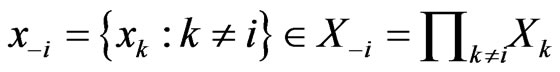 . Similarly, we will use
  to denote any strategy play
  with the type-
 player using strategy
  and his opponents using strategy
 . Thus
  all denote the same play frequencies, and
 . With these notations, the expected payoff for the type-
 players is

Let  be the type-
 player’s
  th pure strategy play with
  having all zero frequencies except for the
  th strategy
 . Then when substituting
  for
for  in the formula above we have the expected payoff for the type-
 players when all of them switches to the
  th pure strategy while its opponents maintain the same plays in frequency:
because  if
if  and
and  if
if .
.
Definition 1 A play frequency  is an Nash equilibrium point if

This means that the type- player will not improve its payoff by switching to any pure strategy from its mixed play frequency
  when other players maintain their Nash equilibrium mixed play frequencies.
Theorem 1 ([17]) Every  -player game has an NE.
Proof. Nash’s proof from [17] is based on a map  with the property that
  has a fixed point by Brouwer’s Fixed Point Theorem and the property that a point is a fixed point of
  if and only if it is a Nash equilibrium point. The definition of
  is as follows. By definition the excess payoff from a mixed play strategy
  for the type-
 player to play his
  th pure strategy is

where , and the total excess payoff (from the mixed play strategy
 ) for the type-
 player is

Notice that  is an NE if and only if
  for all
  and all
  if and only if
  for all
 . The Nash map
  is defined as follows in component for each player:

where . Then it is obvious that
  is a continuous map and is into
  because
 .
.
Let  be any fixed point of
  which is guaranteed by Brouwer’s Fixed Point Theorem. Notice that the type-
 player’s payoff
  is linear in all
  and is a weighted probability average in
 . In fact, we have explicitly

Thus, among all non-zero probability weights  there must be such a
  so that the pure
  -strategy payoff
  is no greater than the mixed payoff
  since otherwise we will have the contradiction that
  because
  and
and . As a result, the corresponding excess payoff is zero,
 . Because it is fixed by
 , we have
 , which must force
  because
 . Since this holds for all
  it shows
  is an NE. The converse is straightforward since the excess payoff from every NE equilibrium
  is zero,
  , which leads to
 .
.
A.2. Mechanistic Derivation of the Nash Map
See the main text.
A.3. Dynamics of the Brown-von-Neumann-Nash Equations for Two-Player Zero-Sum Games
Let  be the payoff matrix for player y with mixed strategy frequency vector
  and
and  be the payoff matrix for player x with mixed strategy probability vector
 . Then the expected payoff for player y is
  and that for player x is
  or equivalently
 . When player y plays its
  th pure strategy, i.e.
  with
with , the corresponding payoff is
 , and hence
  is player y’s payoff vector for all pure strategy plays.
Similarly, player x’s  th pure strategy play payoff is
  and
and  is player x’s payoff vector for all pure strategy plays. Let
  denote the ramp function
  as before. Then the excess payoff for player y’s
  th pure strategy is
  and
and  for all pure strategies in the vector form. Similarly,

is the same for player x’s. And the total excess payoffs are  and
and  , for player y and player x respectively. Let
  denote the simplex for player y's mixed strategy space and
  for player x’s, and
  be the product simplex. Then the corresponding BNN system of equations is
 (6)
(6)
with . For any solution
  of the BNN equation, define the following total excess payoff potential function

The following result is due to [31]:
Theorem 2 Function  is a Lyapunov function for the BNN equation, satisfying

which implies

That is, the convex set of NE are globally asymptotically stable for the BNN equation.
Theorems and proofs of this type were originated by Brown and von Neumann ([18]), and generalized by [31]. Although the proof below for this theorem was a specific case of a generalized theorem (Theorem 5.1) of [31], it is worthwhile to present it here to complete a comprehensive review on the theory of two-player zero-sum games. In addition, the theorem above and its proof below is not readily an obvious special case of Theorem 5.1 of [31], and a stand-alone exhibition should prove convenient for future researchers.
Proof. We first consider only the time-derivatives of those  for which
 . Since
  we have by letting
  and
and 

Using the fact that ,
,  below, we have

Applying the same argument for  we have the following by grouping below the
  terms, of which the mixed term vanishes:

The last equality is due to the following calculations:

since  whenever
 , and similarly we have
 . Hencewe have the following time derivative for
 :
:

As a direct consequence, it follows

and hence the proof of the theorem.
As pointed out previously that the derivation of Nash’s map and the resulting BNN equations suggested an evolutionary mechanism for a two-player zero-sum game to reach its Nash equilibria. The global stability result above indeed proved the case. The next subsection shows on the other hand a Nash equilibria can be found by means of linear optimization, i.e. by the simplex method from linear programming.
A.4. Linear Programming Method for Nash Equilibria of Two-Player Zero-Sum Games
The theory of two-player zero-sum games was first developed by von Neumann in 1928 [32,33]. All results surveyed below are known [15,32-34] but our exposition here seems to be more concise and succinct than all others we know. Our starting point is to assume the knowledge of the simplex method for linear programming.
Here below  are column vectors and
  is a matrix. For two vectors
 ,
,  means the inequality holds componentwise. Also
  denotes the vector of all entries equal to 1 for an appropriate dimension depending on the context. The linear programming (LP) aspect of the two-player zero-sum game theory is based on the following theorem which encapsulates the simplex method and can be found in most linear optimization textbooks, c.f. [35].
Theorem 3 The primal LP problem  subject to
  has a solution
  if and only if the dual LP problem
  subject to
  has a solution
 . Moreover, if they do the solutions
  and
and  must satisfy
 , i.e. the optimal values for both LP problems must be the same.
We note that the optimal solution  for the dual LP problem is referred to as the shadow price or the Lagrange multipliers of the primal LP problem and vice versa. Also, the simplex algorithm for the primal problem will simultaneous find both the optimal solution
  and its shadow price
 . The same for the dual problem as well. For convenience, we also need the following result.
Lemma 1 Let  be the simplex defined by
for all  and
and , then
  . Similarly,
  .
.
A proof is straightforward. In fact, let . Then
  for all
  and since
  we have
  . Hence
 . The equality must hold since the value
  is obtained by the function
  with
with  for
for . A similar argument shows the minimization case.
As before for a two-player zero-sum game,  are the mixed strategy probability vectors, and
  is the payoff matrix for player y against player x. Let
  be the column vectors of the matrix
  and
and  be the row vectors of
 , i.e.
  and
and
 . Then, the expected payoff per play for player y is
 . For a simpler notation we let
 . The bi-linear payoff function
  can be summed in two different ways, each as a probabilistically weighted linear form:
  and
and  for which Lemma 1 will be repeatedly applied below.
Proposition 1  is an NE if and only if

Proof. By definition,  is an NE iff
  for all pure strategy vectors
  of player y and
  for all pure strategy vectors
  of player x since
  is the expected payoff of the latter. That is,
  for all
  and
and . Because
  is a probabilistically weighted linear form in both
  and
and , we have by Lemma 1 that
 .
.
Because both extreme values are reached by an NE point  and
and , the equalities hold. The second equivalence is obvious from the first.□
An NE as a solution  to this optimization problem is also referred to as an optimal game solution or a game solution for short, and
  is referred to as the game value for player y.
Proposition 2 The two-player zero-sum game value is unique.
Proof. Let  be two optimal solutions with game values
 , respectively. Then by the result above,
  because
is an NE for the first inequality and  is an NE for the second inequality. Since
  are two arbitrary NEs, we have by the same argument
 , showing
 .□
.□
Proposition 3 The dual LP problem for the primal LP problem of  subject to
 is
is  subject to
 . Therefore, the optimal value is the same and the solution of one problem is part of the shadow price of the other.
Proof. By introducing  for
for  and
and  and
and  for
for  we can recast the LP problem of
  subject to
  as follows:
  subject to
  for which
  ,
,  ,
,  , and
, and . By Theorem 3, the dual LP problem is
  subject to
  for
for . Writing the latter in
  's block component form, we get
  subject to
  and
and  and
and . Equivalently, let
  we have the dual LP problem reduced to
  subject to
 ,
,  and
and .□
.□
The following two theorems complete our compilation of the basic theory for two-player zero-sum games. The first is the LP algorithm for finding NEs and the second is the maximin theorem.
Theorem 4  is an optimal game solution with the game value
  iff
iff  is a solution to this LP problem:
  subject to
 , and
, and  is a solution to the dual LP problem:
  subject to
 .
.
Proof. Proof of the necessity condition: As an optimal game solution

by Lemma 1, which implies  for all
  and equivalently
 . That is,
  is a basic feasible point for the LP problem
  subject to
 with
with .
.
We claim  must be an optimal solution to the LP problem. If not, there is an
  and
and  such that
  with
with . That is
  componentwise. By Lemma 1, we have
 .
.
Since , this contradicts the property that
  is an NE. Similar arguments apply to the primal LP problem. This proves the necessary condition.
Conversely, because  are the optimal solutions for the dual pair with the optimal value
 , from
  we have
  and from
  we have
  and hence
 . Also, for any
 ,
,  and for any
 ,
,  , showing
  is an optimal game solution with the game value
 .□
.□
Theorem 5 Let  be an NE, then
  over the mixed strategy probability vectors and symmetrically
  .
.
Proof. Notice that the dual LP problem can be equivalently written as

with the smallest such . This implies
  .
.
We claim the equality  must hold. If not, let
  and
and  have the property that
  but
but . Then
  for all
 . In particular,
  , showing
  is a basic feasible point to the LP problem. Since
  is the optimal value of the LP solution, we must have
 , contradicting the assumption
 . Exactly the same argument applies to the primal LP problem.□