Factors Affecting Mode Choice of Work Trips in Developing Cities—Gaza as a Case Study ()
1. Introduction
Gaza strip is located at the southern part of Palestine with area of 365 km2. It consists of five governorates which are: Gaza, Middle, Northern, Khanyounis and Rafah. According to the census conducted by the Palestinian Central Bureau of Statistics (PCBS), the total number of population of Gaza strip at the mid 2011 is 1.59 millions. The percent of males is about 50.6% and the females represent about 49.4% of the populations. According to these figures, Gaza strip is considered one of the most densely populated areas in the world with 4356 inhabitants/km2. The population pyramid for Gaza strip shows that the Palestinian community is a young society where the percent of population in the range between 0 - 14 years is about 44.1% and the populations between 15 - 29 years is about 29.7% while the percent of populations over 65 years represents about 2.4% of the populations. The percent populations within the work age (over than 15 years) represents about 51.7%. The participation of labor force is 38.1% of the populations within the work age. The percent of unemployment is about 40.6% of the peoples within the labor force [1].
Gaza is the densely populated governorate in Gaza strip with a density of 0.75 inhabitants/hectare. The area of Gaza is 7259.3 hectares and the number of population at mid 2011 is 552,000 persons. Gaza city is composed of eleven districts. Gaza has one of the most highly rate of populations increase with a rate of 4% annually. The participation of labor force in Gaza is about 36.4% of the peoples within the work age and the percent of unemployment is about 38.3% [1].
The transport system in Gaza city depends on land transport which can be categorized into private and public transport. Due to the limited income levels in Gaza city, a public transport service plays a major role in satisfying the mobility of the population. The public transport is served by three different modes in Gaza city which are taxi, shared taxi and buses. Taxis are available for point to point transport. Shared taxis are the main mode of public transport services which operate to provide short haul services within the Gaza city. The buses in Gaza city are classified into public and private buses. The registered and licensed public buses serve the regional connection between Gaza city and the other governorates in Gaza strip. Private buses do not have fixed lines but most of its work is directed towards school and university students. As far as private buses are concerned, they do not have stations or terminals and they do not enter the city center regularly.
Before 1994, the transport sector suffered from deterioration in terms of quality and quantity. After signing the Oslo Agreement between Israelis and Palestinians and the establishment of Palestinian National Authority in 1994 there was a dramatic improvement in the construction of road networks. But from another side, there was a high increase in population and vehicles due to the return of a lot of refugees to the Gaza strip. The transport policies adopted by transport planners were not sufficient for solving the transport problems resulting from the increase of travel demands.
Gaza city currently faces urbanization and rapid growth of population, which demands more attention to private and public transport improvements. To meet the increase of travel demands without increasing the congestion problem, there is a need for increasing the use of high occupancy modes, in addition to encourage the use of nonmotorized modes (walking and biking). This could not be done without understanding the travelers’ needs and their preference of using the modes.
In order to adopt suitable transport policies for solving the congestion problem resulting from urbanization and economic growth, there is a need for improving the transport planning process in the Gaza Strip. One aspect that should be improved is mode choice modeling, which is considered very essential for predicting the future growth for each mode, in addition to specifying the factors that contribute to the use of each mode and shifting from one mode to another.
Developing regions including Gaza Strip often utilised the mode choice models that are used in developed countries. These models are not suitable for use in the original form because of the different conditions and circumstances in developing countries. Therefore, there is a need to develop a mode choice model for Gaza in order to help in predicting the future demand of each mode of transport and adopting the suitable transport policies to solve the congestion problem.
This research aims to develop mode choice for work trips in Gaza city that can be used to simulate the behaviour of individuals towards motorized and non-motorized modes. It aims also to determine the factors that affect the employed people’s choice for transport modes.
2. Background
Modeling is one important part of the most decision making process. It is concerned with the methods, be they quantitative or qualitative, which allow us to study the relationships that underlie the decision making [2]. A transport model can be defined as a simplified representation of the real world usually implemented in a computer software, which describes the impact of transport decisions. Transport models can cover whole countries, cities, areas or simply individual junctions. The fundamentals of transport modeling were developed in the united stated during the 1950s’ and imported to the UK in the early of the 1960s’. Thereafter, the following 20 years witnessed important theoretical development in the field of transport modeling leading to further work in specific sub-areas [3].
One of the most important aspects of the transportation modelling is to predict the travel choice behaviour which is the most frequently modelled travel decisions. It involves specific aspects of human behaviour dedicated to choice decisions.
Traditionally aggregate models are used in dealing with the travel choice behaviour of individual travellers; however the aggregate models have the limitation of forecasting and estimating of travel choice with aggregated zone data.
Disaggregate behavioural demand models which became popular during the 1980’s offer substantial advantages over the aggregate counterparts. Disaggregate behavioural models are based on the observed choices behaviour of individual travellers. These models consider that the demand is the result of several decisions of each individual traveller. A discrete choice analysis is the methodology used to analyze and predict the traveller decisions. The discrete choice model is mathematical functions which estimate the probability of individual travel choice based on the utility maximization principle or relative attractiveness of competing alternatives. Revealed and stated preference survey data which contains data sets of individual decisions, characteristics of the individuals and the alternative choices of the trip is used to develop the discrete choice model [4].
There are different factors that affect the choice of transportation modes which can be categorized into three groups. These are factors related to the characteristics of trip maker such as car availability and possessing of driving license; factors related to the characteristics of journey such as, time of day and types of trips; and factors related to characteristics of transport facilities such as cost, travel time and waiting time [4].
There are three types of disaggregate mode choice models namely: logit model, probit model and general extreme value model. Among these types, the logit model is the most widely used for calibrating the mode choice because it is simple in terms of model formulation, in addition to its accuracy compared with the other types [4].
There are many disaggregate mode choice models. Examples of these models are Multinomial Logit [5], Nested Logit [6], Multinomial Probit [7], Generalized Extreme Value [8], Mixed Logit [9] and Multiple Discrete-Continuous Extreme Value [10]. Among these models, Multinomial Logit Model is used in this work because it is the simplest and the most popular discrete choice model as indicated in the literature [4].
The mathematical framework of logit models is based on the theory of utility maximization hypothesis [11]. This hypothesis means that individual selects a mode which maximizes his or her utility [12]. The utility of a travelling mode is defined as an attraction associated to an individual for a specific trip [13]. There are three basic types of logit models depending on whether the data or coefficients are chooser-specific or choice-specific. Multinomial logit model has chooser-specific data where coefficients vary over the choices. Conditional logit model has choice-specific data where the coefficients are equal for all choices. Mixed logit model involves both types of data and coefficients [14].
The logit discrete choice model is mostly derived from the random utility theory. It assumes that each user of transport modes is a “decision maker” and selects to maximize his/her utility. According to [11], common hypotheses are the following:
The individual i considers, in making the choice, all available transportation modes that constitute his/her “choice set”.
The individual i associates to every mode of the choice set a “perceived utility”, which is a function of various attributes, and he/she chooses the mode of maximum utility.
The utility recognized by the individual for every mode is a random variable. This is because the impossibility of correct measuring by an external analyst and because of the characteristics of the individual choice mechanism.
In random utility theory, the relationship between the recognized utility related to each mode j by individual i and the attributes is assumed to be linear [15]:
 (1)
(1)
where

where,  is a function of measured mode-specific and socioeconomic attributes
 ;
;  is unknown random component which represents unobserved attributes, taste variations, and measurement or observational errors;
  unknown parameters;
  is the k-th attribute or variable for mode j belonging to the choice set A_i of individual i;
The probability of choosing maximum utility mode j can be written as [11]:

or more precisely:
 (2)
(2)
Based on the assumption about the joint probability distribution of the set of disturbances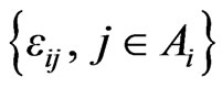 , a specific random utility model can be obtained. In accordance with the Gumbel or Type 1 extreme value distribution, each error
  for the Multinomial Logit Model is assumed to be independently and identically distributed over the population and for each individual. The following cumulative distribution function is used [16]:
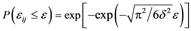 (3)
(3)
with mode zero and variance  for each mode
 .
.
The probability that individual i chooses mode j can now be expressed as [15]:
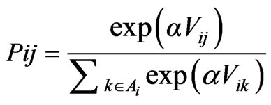 (4)
(4)
The value of  can be taken =1 without any loss of generality in the above equation. This is because
  multiplies all unknown
  parameters according to the
  definition. Thus, estimates of these parameters also include the
  -value.
The method of maximum likelihood is the most common procedure used for determining the estimators in simple and nested logit models. Stated simply as, “The maximum likelihood estimators are the values of the parameters for which the observed sample is most likely to have occurred” [11].
The procedure for maximum likelihood estimation involves two important steps: 1) developing a joint probability density function of the observed sample, called the likelihood function; and 2) estimating parameter values which maximize the likelihood function. The likelihood function for a sample of “I” individuals, each with “M” alternatives are defined as follows [11]:
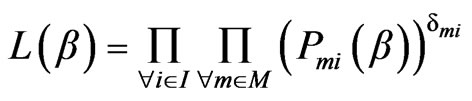 (5)
(5)
where, L is the likelihood the model assigns to the vector of available alternatives;  is the probability that individual i chooses alternative m.
  is chosen indicator (=1 if j is chosen by individual i and 0, otherwise)
The values of the parameters which maximize the likelihood function are obtained by finding the first derivative of the likelihood function and equating it to zero. The most widely used approach is to maximize the logarithm of L rather than L itself. It does not change the values of the parameter estimates since the logarithmic function is strictly monotonically increasing. Thus, the likelihood function is transformed to a log-likelihood function and is given as [11],
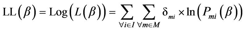 (6)
(6)
The first derivative of the logarithm of likelihood function can be represented as [11]:
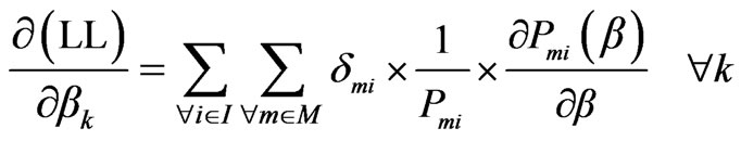 (7)
(7)
The maximum likelihood is obtained by setting (7) equal to zero and solving for the best values of the parameter vector, . To insure this is the solution for a maximum value provided that the second derivative is negative definite.
Given the mode choice data, most existing estimation computer programs estimate the coefficients that best explain the observed choices in the sense of making them most likely to have occurred. Standard commercial packages such as ALOGIT and Easy Logit Modeler (ELM) are generally used for estimating logit models, mostly due to their capability of handling complex nested logit structures, both linear and non-linear.
3. Methodology
In order to achieve the objectives of this study the work is divided into six phases. The first phase is the literature review on mode choice modeling. The second phase relates to the process of selection of the travel attributes. It involves, designing of initial (pilot) questionnaire and analysis of the survey data to determine the attributes which are most relevant to the travelers in the study area. The third phase involves designing the final questionnaire and conducting the survey. It includes selection of level of attributes; determining the sample size and sample space; implementation of the survey; and collection and analysis of data. The questionnaire is divided into three parts. The first part includes the socio-economic information about the respondents such as (gender, age, job, income, family size, ownership of private car, ownership of motorcycle, ownership of bicycle… etc). The second part focuses on the factors that affect the mode choice. The respondents were asked to indicate their perception on the importance of twelve factors that affect the choice of transportation mode for work trips in Gaza city. These variables are: age, gender, average monthly income, travel cost, travel time, waiting time, weather conditions, privacy, comfort, health status, and trip length. A five point Likert scale (ranging from 1: very low important to 5: very high important) was adopted to analyze the importance of factors that affect the choice of transportation mode. The third part focuses on the trip characteristics. For the purpose of this study, the daily trips which constitute home-work trips have been included. In this part, the information covered is related to travel behavior of individual for his/her daily trips such as (the mode usually used, travel time, travel cost, monthly fuel consumption, license and maintenance cost, etc.). For the purpose of this study, 700 questionnaires were distributed for work trips. The random sample method was adopted in this study. Of the 700 questionnaires were distributed, 552 questionnaires are valid. Two thirds of these questionnaires were used for calibration of model and the rest were used for the validation process. The fourth phase includes calibrating and estimating of the utility functions for the Models. The best model is chosen by comparing the models with regard to the coefficient estimates of the variables and their overall goodness of fit. The fifth phase is preliminary concerned with the model validation. The validity of the model was tested by Likelihood Ratio Test (LRTS) and estimation of prediction ratio. The null hypothesis formulated for the purpose is as follows:
H0: there is no difference between the observed and predicted behaviour i.e. there is no difference between the parameter vectors obtained from calibration data and the validation data H0: βi = βjwhere βi, βj are the estimated parameter vectors of the model obtained from calibration and validation data (the same specification is needed for this test).
To obtain the LRTS value the coefficient of variables of particular model will be restricted and the ELM program is executed with validation data. The program outputs two log-likelihood values. The first value is the one computed by restricting the coefficient of the calibrated model while the second is the one when the parameters are unrestricted for validation data. The LRTS value can be obtained by the following equation [15]:
 (8)
(8)
where,  represents the likelihood ratio test statistics which restricts the parameters estimated from data j to be used to predict mode share in data i for same specifications;
  is log likelihood ratio value when the parameters are restricting in data j;
  is log likelihood ratio value when the parameters are unrestricted in data j.
The LRTS tests discussed is distributed as chi-square with k degrees of freedom where k is the number of model parameters. If LRTS value is less than critical chi-square value @ 95% confidence level and degree of freedom equal to k then for that particular case the null hypothesis can’t be rejected otherwise it is rejected. The last phase summarizes the main findings and conclusions from the study.
4. Results and Analysis
This section is divided into three parts. The first part presents the general analysis of data. The second part includes calibrating and estimating of the utility functions for the different models and then choosing the best model. The third par concerns model validation.
4.1. General Analysis of Data
Initially, frequency tables were obtained on a whole datasets to determine the distribution of travellers for various travel and socioeconomic characteristics. The results of this analysis are summarized in Table 1.
4.2. Calibration of Revealed Model
On the basis of descriptive analysis of the data, there are six modes to be considered for modeling the mode choice for work trips in Gaza city which are private car, shared taxi, taxi, motorcycle, bicycle, and walking.
Different specifications have been evaluated to determine which one will replicate the data for work trips in Gaza city. The list of variables that have been used in model calibration with their abbreviations is presented in Table 2.
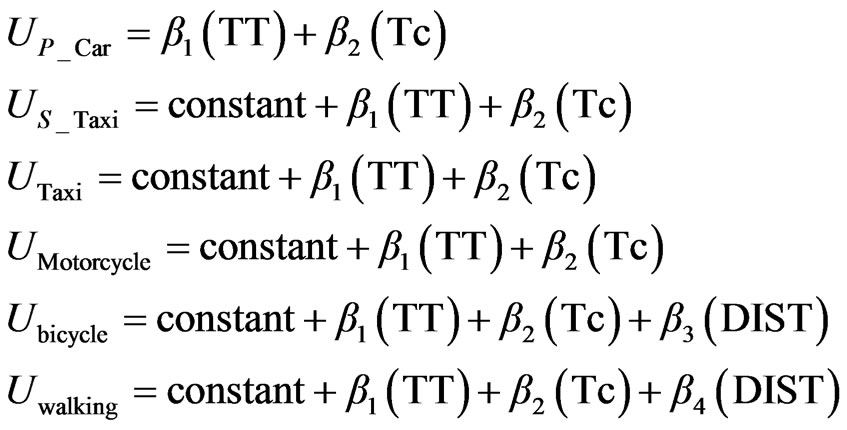
The first model which has been built includes total travel time (TT) and total travel cost (TC) as generic variables which means that an increase of one unit of travel time or travel cost has the same impact on the modal utility for all modes. The distance variable (DIST) considered as a specific variable for bicycle and walking modes. The private car mode was considered as a base mode when adding constants for the mode utilities. The utilities for different modes can be written as the following:
 (9)
(9)
The obtained results shown in Table 3 illustrate that the estimated coefficients of cost and travel time variables have a negative sign, as expected, which means that the utility of modes decreases as the travel time and travel cost increase. The results also show that both travel time
(TT) and distance for walking (DIST) have a large absolute values of t-statistics of 2.764 and 3.82 respectively which are greater than critical t-value at 90% confidence level (1.65). This result leads to the rejection of the null hypothesis that these variables have no effect on modes utilities. Although the t-statistics of travel cost variable is a little bit lower than critical t-value at 90% confidence level, it should be included in the model because it considered as a policy variable [4]. The lack in significance of the alternative specific constants for shared taxi, taxi, motorcycle and bicycle is immaterial since the constants represent the average effect of all variables not included in the model and always should retain in the model despite the fact they do not have well understood behaviour interpretation [17]. The t-statistic on bicycle specific distance variable is less than critical t-value even at 90% confidence level. This suggests that the effect of distance on bicycle utility may not differentiate it from the reference mode (private car mode), so this variable is considered to be dropped from the model.
The removing of distance variable (DIST) from the utility of bicycle leads to model_2, where the utility of bicycle can be written as the following while the utilities for the other modes still the same as in model_1:
 (10)
(10)
The obtained results for model_2 can be shown in Table 3. The results for the two models show that both have a good goodness of fit measures ρ2. To compare the two models, a likelihood test was applied in order to study the impact of exclusion a distance specific variable from the utility of bicycle mode. The null hypothesis to be tested stated that there is no impact of a distance specific variable on the mode choice decision:
 (11)
(11)
The statistical test that a distance specific variable (DIST) for bicycle mode has no effect on the choice decision has a chi square value of
 (12)
(12)
where, LLR is the log likelihood of the restricted model; LLU is the log likelihood of the unrestricted model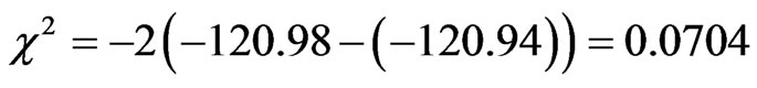 .
.
With one degree of freedom (one variable was constrained to zero), the null hypotheses can’t be rejected even at low confidence level of 90%. The chi square value is << critical chi square value at 90% confidence level (2.71). Thus, the distance specific variable can be excluded from the bicycle utility.
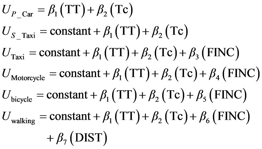
In order to improve the statistics of model_2, new intuitive variables were added to the model. Average monthly income for family variable (FINC) was added to the utility function of taxi, bicycle, motorcycle and walking and the model was estimated and labelled as model_3. The utility functions for different modes can be written as the following:
 (13)
(13)
The results presented in Table 3 illustrate that both travel time and travel cost variables have a correct negative sign of coefficients and they are statistically significant at 90% confidence level, where the t-statistics value are greater than the critical one (1.645). The results also show that both average family monthly income variables for taxi and bicycle are statistically insignificant at significance level greater than 0.1, where the t-statistics value is less than the critical one at 90% confidence level. Therefore, the null hypothesis that these variables have no effect on choice decision can’t be rejected even at 90% confidence level so these two variables are suggested to be dropped from the mode. The dropping of average family monthly income variable (FINC) from the utility functions of bicycle and taxi modes leads to new model labelled as model_4 where the utilities of taxi and bicycle modes can be written as the following while the utilities for the other modes still as they were in the previous one.
 (14)
(14)
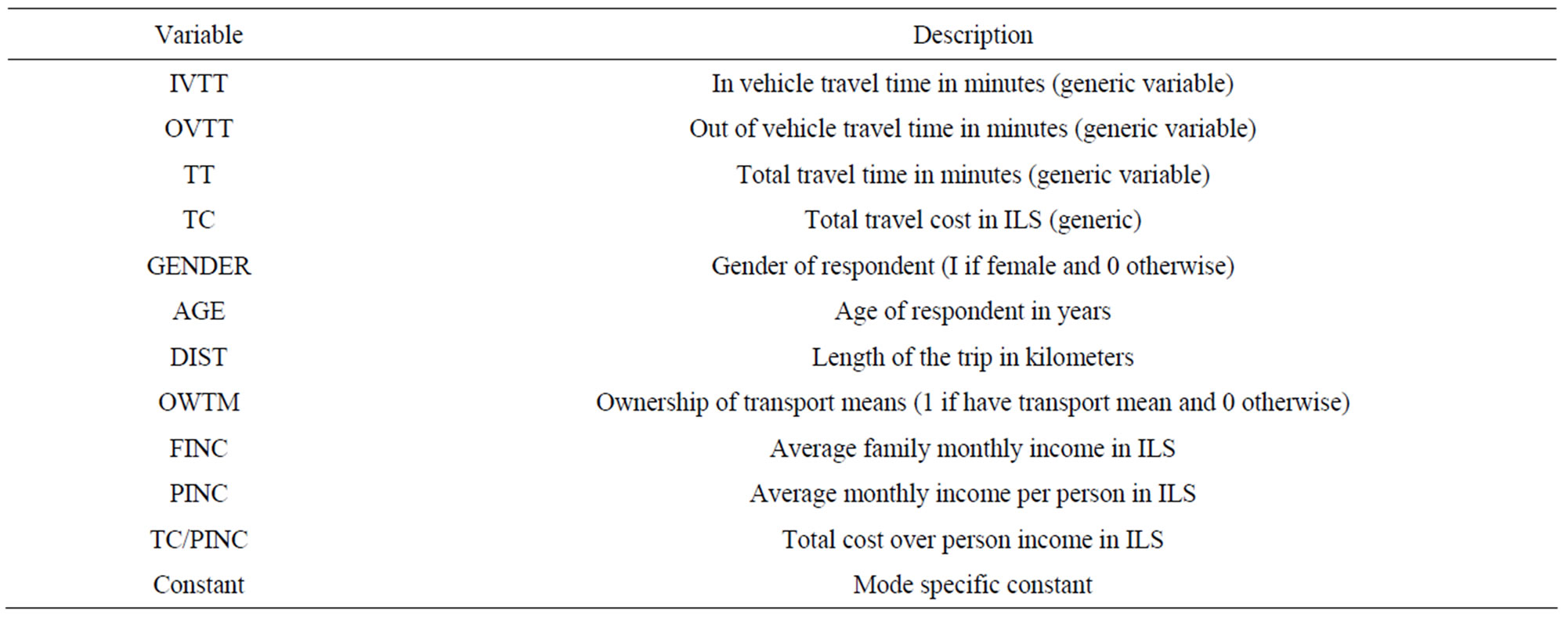
Table 2. Description of explanatory variables.
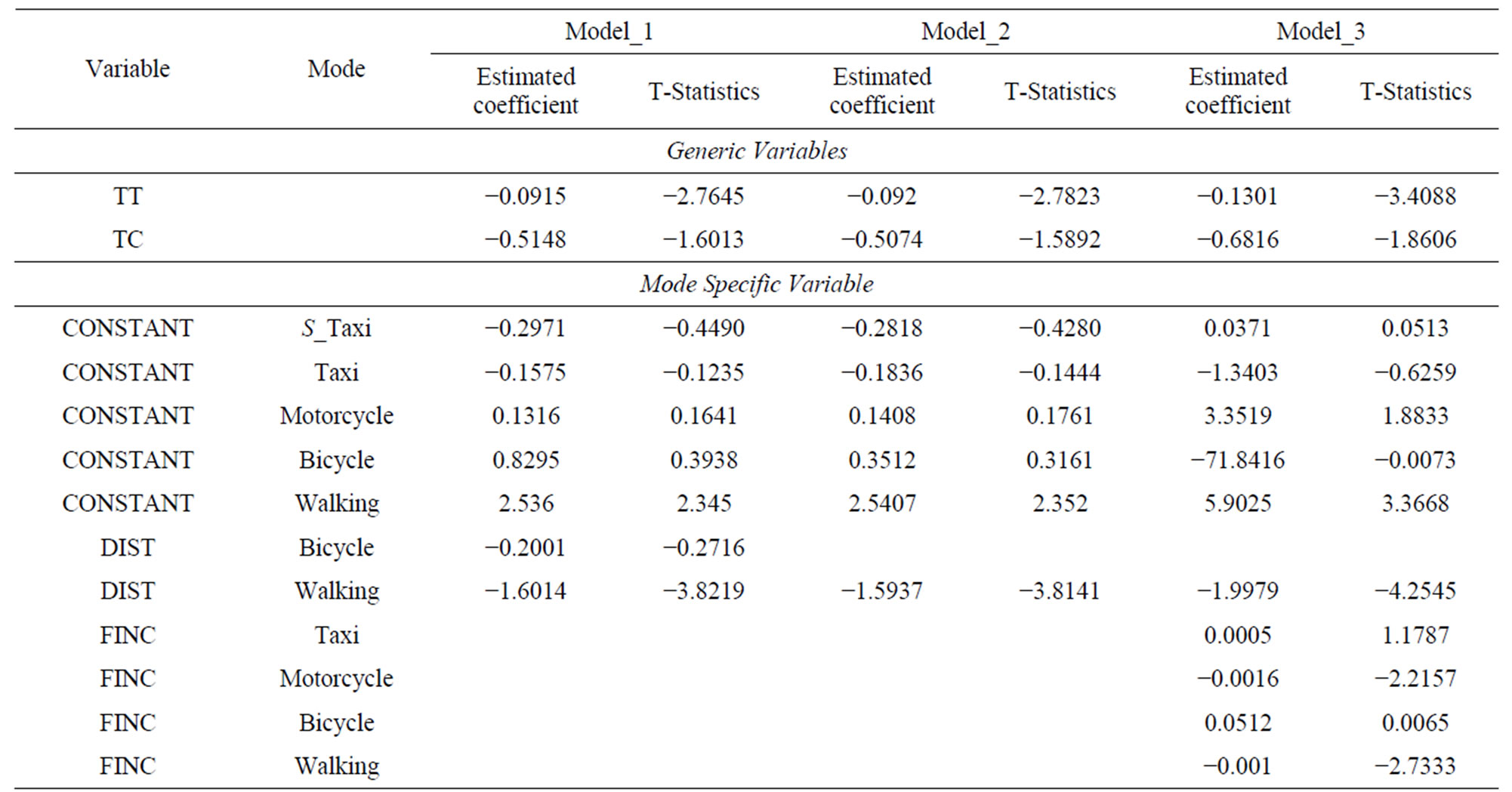
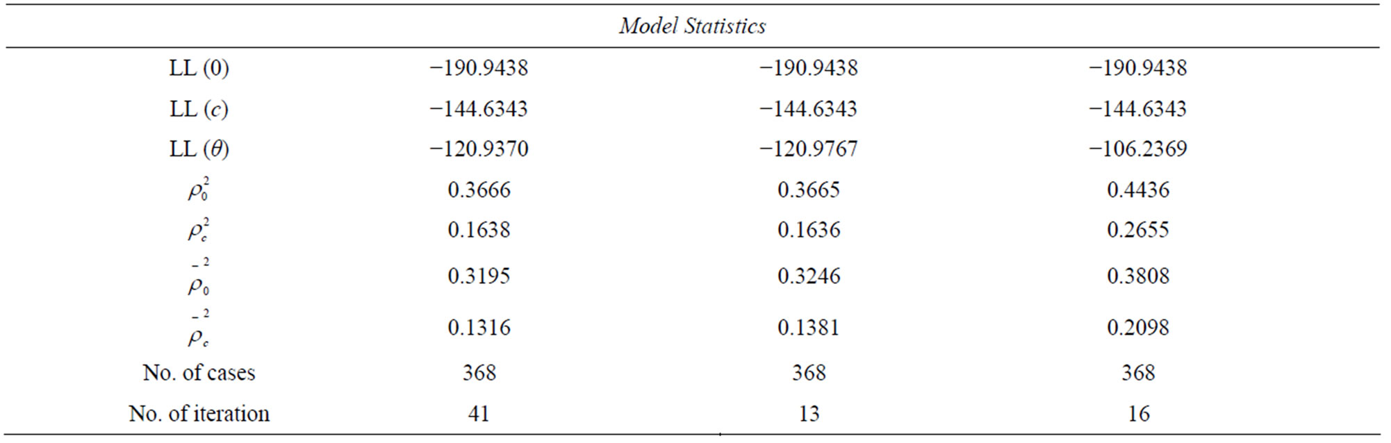
Table 3. Estimation results of Model_1, Model_2 and Model_3.
The results for the model mentioned above are reported in Table 4. The results reported in the Table show that both travel time and travel cost have negative sign of coefficients as expected. The results also show that travel time (TT), distance (DIST), average family monthly income for motorcycle (FINC motorcycle), and average family monthly income for walking (FINC walking) have absolute t-statistics value of 2.98, 4.17, 2.38, and 3.14 respectively, which are greater than the critical t-value at 95% confidence level. Therefore, the null hypothesis stated that these variables have no effect on choice decision and can be rejected at significance level greater than 0.05.
Even though the travel cost variable (TC) has a low absolute t-statistics value of 1.51, which is less than the critical t-value even at 90% confidence level, it will retain in the model because it is considered as level of service variable. In order to study the effect of adding average family monthly income variable to both motorcycle and walking utilities on the statistics measures of the model, this model was compared with model_2. The comparison of the two models show that the goodness of fit measures for this model ,
,  ,
,  and
and  were improved to 0.405, 0.2145, 0.3526, and 0.1739 compared with 0.3665,
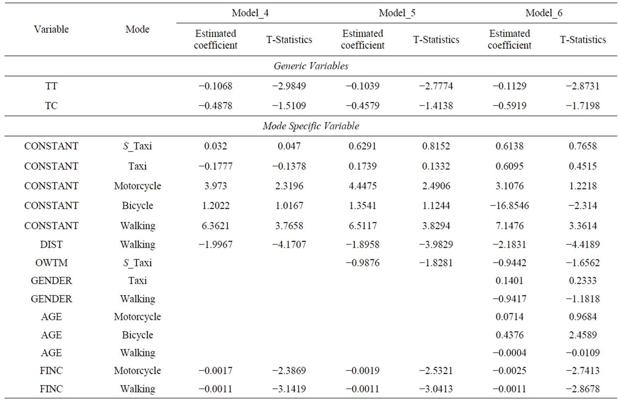
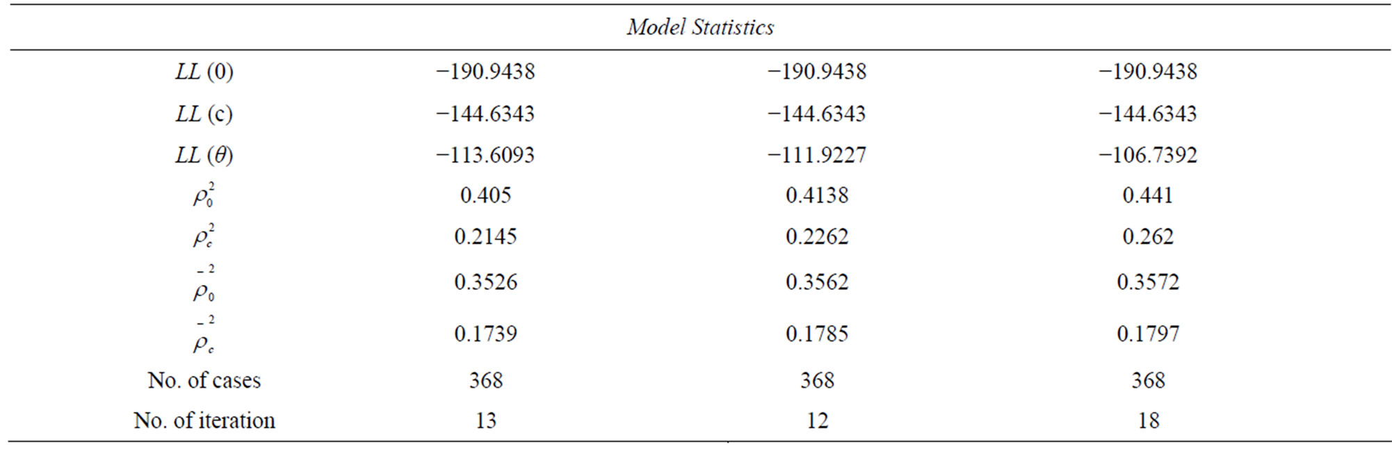
Table 4. Estimation results of Model_4, Model_5 and Model_6.
0.1636, 0.3246, and 0.1381 for model_2. For further improvement of the statistics of model_4, the ownership of transport means variable (OWTM) was added to the utility of shared taxi and the new model was labelled as model_5. The utilities for different modes can be written as the following:
 (15)
(15)
Table 4 presents the results of the model. As can be seen from the table, both travel cost and travel time coefficients have a correct negative sign. The results also show that the total travel time (TT), ownership of transport means (OWTM S_taxi), distance (DIST walking) and average family monthly income for motorcycle and walking modes (FINC Motorcycle, FINC Walking) variables have a large absolute t-statistics values of 2.774, 1.828, 3.98, 2.53, and 3.04 respectively, which are greater than the critical t-value at 90% confidence level (1.645). This result leads to reject the null hypothesis stated that these variables have no effect on choice decision. Although total cost (TC) variable has absolute value of t-statistic (1.4138), which is lower bit than critical t-value at 90% confidence level, it will retain in the model as it is considered as a policy variable. The goodness of fit measures for this model ,
, ,
,  and
and  were improved to 0.4138, 0.2262, 0.3562, and 0.1785 compared with 0.405, 0.2145, 0.3526, and 0.1739 for model_4.
To study the hypothesis involving with the exclusion of OWTM variable from the model, the likelihood ration test was applied between model_4 and model_5. The null hypothesis to be tested stated that the OWTM variable can be excluded from the model.
 (16)
(16)
The statistical test has a chi square value of  thus the null hypothesis can be rejected at significance level greater than 0.1 and one degree of freedom (one variable OWTM was constrained to zero). According to this result, the OWTM variable has to be retaining in the model.
To study the effect of social characteristics on mode choice, gender variable (GENDER) was added to both taxi and walking utilities and the age variable (AGE) was added to motorcycle, bicycle and walking utility functions. The new model was labelled as model_6 with the following utility functions:
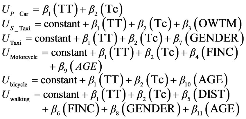 (17)
(17)
The results for this model were reported in Table 4. The results show that the travel time and travel cost variables have a correct sign of estimators and they are statistically significant at 90% confidence level, where the t-statistics value is greater than the critical one. The results also show that the OWTM S_taxi, DIST walking,, FINC motorcycle, FINC walking, and AGE bicycle are statistically significant at significance level greater than 0.1 with a t-statistics values of 1.65, 4.4189, 2.7413, 2.8678, and 2.4589 respectively. Thus, the null hypothesis that these variables have no effect on mode choice can be rejected at significance level greater than 0.1. Gender variable for both taxi and walking modes and age variable for motorcycle and walking modes are statistically insignificant at 90% confidence level as the t-statistics for these variables have values of 0.2333, 1.1818, 0.9684, and 0.0109, which are less than the critical t-value at 90% confidence level (1.645). Hence, the null hypothesis that these variables have no effect on choice decision can’t be rejected at the specified significance level. Thus, these variables are suggested to be excluded from the model. The exclusion of gender variable from the utility functions of taxi and walking modes, in addition to the exclusion of age variable from the utility functions of motorcycle and walking modes leads to new model labelled as model_7. The results for the model which were reported in Table 5 show that all the variables have a correct sign of estimators and they are statistically significance at a confidence level of 90%, as the t-statistics for them are greater than critical t-value at significance level greater than 0.1. Therefore, the null hypothesis stated that these variables have no effect on choice decision can be rejected at that confidence level.
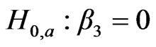
In order to test the hypothesis involving with exclusion of gender variable (GENDER) from the utility functions of taxi and walking modes, in addition to exclusion of age variable from the utility functions of motorcycle and walking modes, the likelihood ratio test was applied between model_6 and model_7. The null hypothesis can be written as the following:
 (18)
(18)
The statistical test has a chi square value of
 ,
,
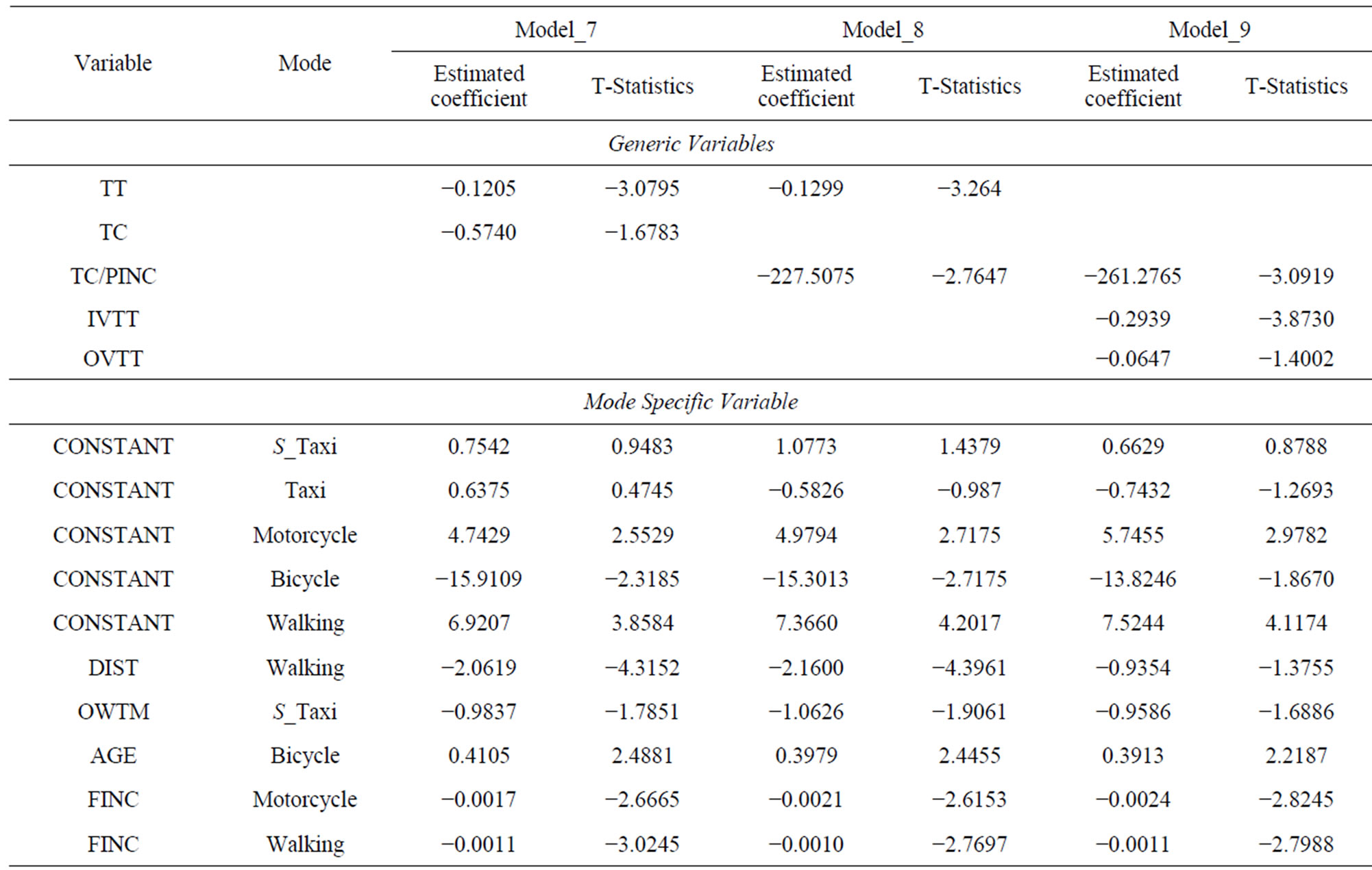

Table 5. Estimation results of Model_7, Model_8 and Model_9.
which is less than critical chi square value at significance level greater than 0.1 with four degrees of freedom (four variables were constrained to zero) (7.78). According to this result the null hypothesis can’t be rejected even at 90% confidence level, therefore these variables seem to have no effect on choice decision.
For studying the possibility of excluding age variable from the utility function of bicycle mode, the likelihood ratio test was applied between model_7 and model_5. The statistical test has a chi square value of
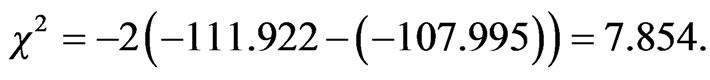
with this condition the null hypothesis that this variable can be excluded from the model can be rejected even at significance level greater than 0.01 with one degree of freedom as the chi square value (7.854) is greater than the critical value (6.63).
The decision maker related variables such as average income, ownership of transport means, family size and others can be included in the models by two approaches. The first is to include them as specific variables to each or some of alternatives (except for the reference alternative). All the models reported to this point used this approach for inclusion of decision maker related variables in the models. The other approach is to include such variables through interaction with mode attributes such as dividing cost by income to reflect decreasing the importance of cost by increasing the annual income.
To take this issue into account, the travel cost variables in the previous model (model_7) was replaced by cost over person income variable (TC/PINC). The new model was labelled as model_8 with the following utility functions:
 (19)
(19)
The results which are presented in Table 5 show that travel time and cost over personal income variables have a correct sign of estimators. The results also show that except ownership of transport means (OWTM) which is statistically significant at 90% confidence level, all the variables are statistically significant at significance level greater than 0.05, as they have an absolute value of t-statistics larger than critical t-value at 95% confidence level (1.96). This result leads to the rejection of the null hypothesis that these variables has no effect on choice decision at significance level greater than 0.1 (90% confidence level).The goodness of fit measures for this model
 ,
, ,
,  and
and  were improved to 0.4454, 0.26790.3826, and 0.2122 compared with 0.4344, 0.2533, 0.3716, and 0.1981 for model_7 respectively.
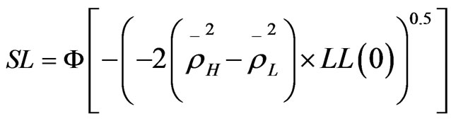
To compare model_7 with model_8, a non-nested hypothesis test was applied for this purpose as the two models have the same number of variables. The null hypothesis to be tested stated that the lower roh-square model is the true model. In non-nested hypothesis test the adjusted roh-square is used to test the hypothesis. The null hypothesis can be rejected at significance level SL determined by the following equation:
 (20)
(20)
where,  is the adjusted roh-square relative to the zero model with higher value.
  is the adjusted roh-square relative to the zero model with lower value.
  is the standard normal cumulative distribution function.
As model_8 has better goodness-of-fit than model_7, then the null hypothesis to be tested is that the model_7 is the true model. The significance level to reject the null hypothesis can be calculated as follows:
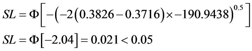
As the significance level calculated from the equation above is less than 0.05 then the null hypothesis that model_7 is the true model can be rejected at significance level greater than 0.05. The result is consistence with the theory that the importance of travel cost decreases as the income increases.
The above formulated models assume that the utility of in vehicle travel time (IVTT) and out of vehicle travel time is (OVTT) are equal; however the workers may be more sensitive to one of them than the other. In order to take this issue into account the total travel time was disaggregated into two parts namely in vehicle travel time and out of vehicle travel time and a new model was formulated with the following utilities:
 (21)
(21)
The new model was labelled as model_9 and the results for the model can be seen in Table 5. The results shown in Table 5 show that in vehicle, out of vehicle travel time, and total travel cost variables have a correct negative sign of estimators. The results also show that all the variables except out of vehicle (OVTT) and distance variables (DIST) are statistically significant at 90% confidence level, where the absolute value of t-statistics are greater than critical t-value (1.645) so that the null hypothesis that these variables have no effect on choice decision can be rejected at level of significance greater than 0.1. Although OVTT, and DIST are statistically insignificant at 90% confidence level, caution should be taken before removing it from the model as its dropping may adversely affect the significance of other variables.
As can be seen from the results, the in vehicle travel time has a larger coefficient than out of vehicle travel time , this results contradict with the results of some researches such as [18] which concluded that the travellers are more sensitive to out of vehicle travel time than in vehicle travel time. The good accessibility for the trips in Gaza city and the short access, egress and waiting time of the trips may explain this result.
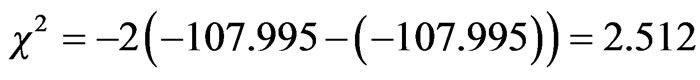
The test of hypothesis of equal value of in and out of vehicle travel time, the likelihood ratio test was applied between model_8 and model_9. The statistical test has a chi square value of
 .
.
This result leads to reject the null hypothesis and accordingly reject the constraints imposed by model_8 at a significance level greater than 0.05 with one degree of freedom as the chi square value calculated above is larger than the critical chi square value at 95% and one degree of freedom (3.84).
By comparing the above formulated models, it is clear that model_8 and model_9 have the best goodness of fit measures among the estimated models. Model_9 has goodness of fit measures ,
, ,
,  and
and  of value 0.4647, 0.2934, 0.3967, and 0.2301 respectively which is better than the goodness of fit measures for model_8 which has a goodness of fit measures
 ,
, ,
,  and
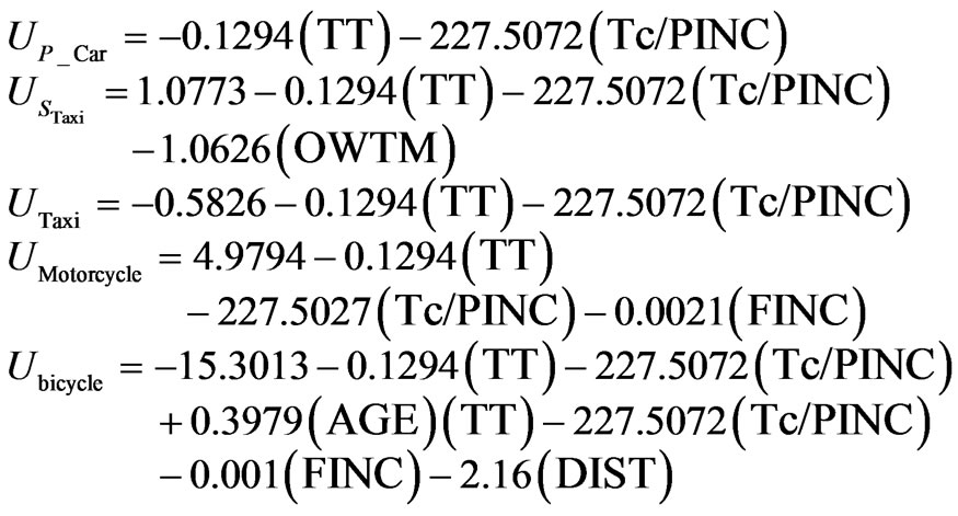
and  of 0.4454, 0.2679, 0.3826, and 0.2122 respectively. Although Model_9 is better, it suffers from a shortage represented on that some of variables in this model (out of vehicle (OVTT), and distance (DIST) are statistically insignificant even at 90% confidence level. So, based on the criteria which were mentioned in the methodology for comparing the models and choosing the most satisfactory one, model_8 seems to be the most satisfactory one for representing the behaviour of employed people in choosing the mode of transport in Gaza city, as this model has a correct sign of estimators and all the variables are statistically significant at 90% confidence level. In addition, it has a good goodness of fit measures, while some of variables in model_9 (which is better than it in goodness of fit measures) are statistically insignificant at 90% confidence level. The utility functions for the model can be written as following:
4.3. Validation
Model validation is considered very important process to evaluate the performance of the calibrated model and its ability to predict modal split for data other than that used for calibration process. The validation process is tested on three different phases. The first phase is the test of reasonableness validation process which was tested during the calibration process depending on the expected sign of estimators. All models with a wrong sign of estimators would not consider as a valid model. Based on this criterion, it is clear that model_8 which was chosen as the most satisfactory model for work trips in Gaza city is considered as a valid model because the travel time and travel cost variables have correct sign of estimators (negative signs).
The second phase of validation process is the statistical validation test which is conducted by the likelihood ratio test (LRTS). This test was conducted for model_8 using about 1/3rd of the data sets (184 observations). The results of this test show that the calculated chi square was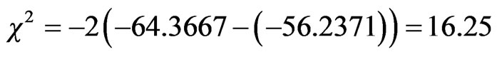 . With twelve degrees of freedom (number of restricted coefficients) as indicted in equation 19, the calculated chi square value can’t lead to the rejection of the null hypothesis stated that there is no difference between the predicted and observed behaviour because the calculated chi square value is less than critical chi square value at 95% confidence level and twelve degrees of freedom (21.026).
The last phase for validation process is calculated the prediction capability of the calibrated model (model_8). To calculate the prediction ratio, the utility for each trip maker was calculated, then the probability of each alternative (mode) was estimated. The alternative with the highest probability is predicted to be the chosen mode for that particular. The number of travelers correctly predicted was summed up to each alternative and compared to yield the prediction value. The calculated prediction value was 0.69 which means that the model is capable to predict about 69% of the choices of the trip makers’ correctly.
5. Conclusions and Recommendations
Based on the findings of the research, it is found that, the total travel time, total travel cost divided by personal income, ownership of transport means, age, distance and average family monthly income are the factors that affect the mode choice of employed people in Gaza city. As the gender and out of vehicle time are statistically insignificant at 90% confidence level, they were excluded from the model. The developed model is able to predict the choice behaviour of employed people in Gaza city as they are valid at 95% confidence level. Several recommendations have emerged from this research. 1) The developed model can be used in travel demand analysis and in developing transport policies for Gaza city; 2) awareness campaigns should be implemented to encourage young people for using a bicycle mode; 3) further studies should be used for developing mode choice models for trips other than work trips such as social, recreational and study trips; 4) the effect of captive travellers on mode choice models should be studied; 5) the mode choice should be modelled using probit and generalized extreme model and compared with logit model.