High Dimensional Dataset Compression Using Principal Components ()
1. Introduction
Principal Component Analysis (PCA) has been used extensively in the atmospheric sciences for over 60 years [1-4]. The value of PCA in atmospheric sciences applications stems from the compact description of space-timevariable datasets into two graphical displays that convey the dominant patterns of space variation and their associated time behavior. One challenge of using PCA is its high computational time complexity. Numerical models often measure variables on grids of L latitudes by M longitudes by N vertical levels, with LxMxN gridpoints, with model output at T times. This leads to a data matrix of either T x (LxMxN) or (LxMxN) x T for each model variable, P.Since LxMxN is often of order 108, an eigendecomposition of the model output can be a daunting task, since PCA requires O((LxMxNxP)3) computations. With ten variables typically being analyzed simultaneously, this can lead to matrix diagonalizations of the order 109.
The models are expected to exceed 1010 in the near future.
To make such high dimensional applications more tractable, several methods have been developed, such a block PCA [5], where the data are divided into blocks and the leading eigenstructures are drawn for each block and reassembled to reconstruct the data with a relative small number of PCs. The scheme has been shown to have promise for reconstructing data, such as human faces [6]. However, in meteorology, the individual eigenstructures are often interpreted as the dominant modes of variability or teleconnection patterns [7], making block PCA less attractive. If the dimension T << (LxMxNxP), the data may be analyzed in the T-dimension or a singular value decomposition [8] can be used to extract the T eigenvalues and eigenvectors. Whereas these approaches have merit in certain applications, they assume that the T-dimensional decomposition contains the eigenstructures of interest, as either the variability is limited to the time dimension or the eigenvalues are drawn from the smaller time dimension of the data matrix, leading to a limited number of eigenmodes. In the present application, we seek to analyze the (LxMxNxP) dimension to determine groupings of those variables that have similar time evolutions for severe weather outbreak types [9-12]. In so doing, we obtain modes of variability in the three-dimensional atmosphere that corresponds to 24 hours prior to the onset of severe weather, useful to forecasters. Forecasting severe weather a day before it occurs is controlled largely by atmospheric spatial scales exceeding approximately 2000 km in distance (referred to by meteorologists as synoptic scale or larger). Data over such an area represent a nearly instantaneous snap-shot of the state of the atmosphere and the features at this scale tend to persist long enough to enhance predictability. If the validity of eigenstructures at these space scales is established, they can be investigated as precursors of the outbreaks. Knowledge of such patterns can assist in forecasting the location of the severe weather a day or more in advance of the outbreak, thereby providing the potential to reduce casualties.
2. Data and Methods
2.1. Defining Outbreaks
Prior to formulating composites of the different outbreak types, a formal definition of each outbreak type was required. Following the ranking methods outlined in [13], the N15 ranking index of outbreaks was used to assess significant tornado outbreaks. In particular, outbreaks with an N15 ranking index of 2 or higher that included 6 or more Storm Prediction Center (SPC) tornado reports were considered as “major” tornado outbreaks. However, since the N15 ranking index was developed based on criteria relevant for tornado outbreak severity (e.g. the number of tornadoes that cause death, the number of significant tornadoes, etc.), using this scheme for ranking hail and wind-dominated outbreaks was not appropriate. Since no formal ranking approach exists for these outbreak types, a simple relationship comparing the number of wind reports and hail reports was utilized to define each group. In particular, outbreaks whose number of wind reports exceeded three times the number of hail reports that had an N15 ranking of less than 2 (thereby excluding them from the tornado group) were considered “major” wind outbreaks, while outbreaks with three times the number of hail reports as wind reports with an N15 index < 2 were considered “major” hail outbreaks. Through the use of these criteria, sets of 79 tornado outbreaks, 131 wind outbreaks, and 245 hail outbreaks were defined for the time dimension.
2.2. Data and Analysis Procedure
High dimensional studies require some modification of the typical eigenanalysis methodology. Prior to the data reduction, rather than examining scalar values, graphical methods are employed where possible. The steps in the analysis are: (1) decision on the type of analysis dictated by research question, (2) sampling available data, (3) quality control and missing data, (4) remapping the data to an unbiased grid, (5) scaling the data, if necessary, (6) formation of a similarity matrix, (7) diagonalization of similarity matrix, (8) selecting a range of the number of eigenvectors, (9) formation of unrotated principal component loadings, (10) rotation of different numbers (from step 7) of unrotated PC loadings to select the most appropriate number of rotated PC loading vectors, (11) extraction of rotated PC scores and (12) physical interpretation of the results.
Step 1. Our research goal is to identify recurring patterns of atmospheric variables associated with tornado, hail and wind severe weather outbreaks. This is a spacetime analysis of the three-dimensional atmosphere and we form a multilevel set of grids in the data matrices, with the spatial gridpoint values of the variables as columns and the outbreak cases as rows. The NCEP/NCAR reanalysis project (NNRP) [14] provides three-dimensional global reanalyses of numerous meteorological variables, relevant to severe weather formation. The dataset is defined by a horizontal (LxM) 2.5˚ latitude-longitude grid spacing with 17 vertical levels (N) and over the entire globe at 6 hour time intervals from 1948 to present. For this study, three-dimensional fields of geopotential height, specific humidity, zonal and meridional wind components, were obtained for a study domain centered on North America (Figure 1) for each outbreak type. Four of the variables: geopotential height, temperature, zonal and meridional wind were measured at all 17 levels (4 × 17 = 68 of the 83 variables). The specific humidity data are not provided at pressure levels less than 300 hPa; therefore, the eight levels closest to the surface were selected. Additionally, there were seven surface variables (mean sea-level pressure, surface pressure, temperature, zonal and meridional wind components for a total of 68 + 8 + 7 = 83 variables for each gridpoint. Variables were obtained 24 hours prior to the valid time of the outbreak to construct each outbreak type matrix (i.e., tornado, hail, wind). Hence, these matrices provide information on the pre-outbreak atmosphere, a time frame that is particularly useful to severe weather forecasters or pattern recognition algorithms looking for outbreak precursors.
Step 2. Data from the beginning of the NNRP record until the last date available were used in this study. Therefore, our sample is the finite population of all reanalysis data.
Step 3. There were no missing data and the reanalysis has been subject to extensive quality control prior to our analysis. Therefore, the data were not adjusted.
Step 4. The NNRP are provided on a latitude-longitude grid (Figure 1(a)). The goal of the analyses is to provide modes of variability of the spatial coherence of the data. Owing to the poleward convergence of the longitude lines in the NNRP data, there is an artificial inflation of association among nearby gridpoints (i.e., their covariances) that is a function of latitude. As eigenanalysis is a decomposition of the variance structure of the data, it is necessary to remove this source of bias by interpolating to a Fibonacci grid [15] (Figure 1(b)), by providing equally spaced gridpoints over the entire domain (318 Fibonacci gridpoints). Three final datasets resulted from these analyses, consisting of all gridpoints (ordered longitude-latitude-level-variable) along the columns of each matrix (26,394 columns) and the events on the rows (numbers match number of outbreaks of each type). This defines an S-mode analysis [16].
Step 5. Because the variables have vastly different units and values (e.g. specific humidity ~ 1 × 10⁻³ kg/kg versus geopotential height at 500 hPa ~ 5400 m), the data were pre-standardized through z-score calculations ateach vertical level and for each variable prior to place
 (a)
(a) (b)
(b)
Figure 1. The study domain on the original NNRP grid (a) and on the Fibonacci grid (b).
ment in the data matrices that were to be eigenanalyzed. Since the data were standardized to a zero mean and unit standard deviation at each vertical level to account for the varied units and large variation in the values as a function of pressure level, values in the data matrices are standardized anomalies (Z).
Step 6. As values in the data matrices are standardized anomalies (Z) from the mean (step 5), similarity is measured by forming correlation matrices (R) of order 26,394. Three correlation matrices are formed for tornado, hail and wind outbreaks.
Step 7. Each correlation matrix was decomposed into a square matrix of eigenvectors (V) and associated diagonal matrix of eigenvalues (D), given by the decomposition
 (1)
(1)
Step 8. The rank of the eigenvector matrix is equal to the smaller of the number of gridpoints (n) or number of observations (m) minus 1. Because there were m = 79 observations for tornado outbreaks, only 78 eigenvalues were nonzero and 78 eigenvectors were extracted. Similarly, 244 (130) non-zero eigenvalues existed for the hail (wind) outbreaks. The goal of this stage of the analysis is to create a set of basis vectors that compress the original variability in R into a new reference frame. It is possible to plot the n elements of each eigenvector (V) on spatial maps; however, the patterns in V do not result in any localization of the spatial variance, nor do they represent well the variability in R [16].
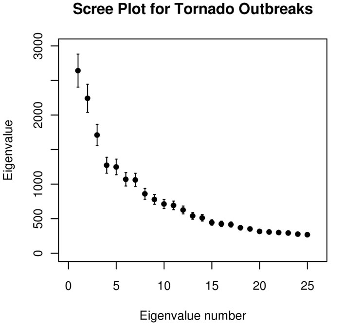
For high dimensional problems, interpretation requires that the analyst must explain the relationships among many thousands of variables for each eigenvector retained. The eigenvectors are ordered indexed by decreasing eigenvalue. Many of the 78 eigenvectors depict smallscale (sub-synoptic scale) signals with variance properties indistinguishable from noise, having very small eigenvalues. We truncate the number of principal components to represent only that variance associated with synoptic scales or larger that correspond to spatial patterns present in the 26,394 × 26,394 correlation matrix, using a two step process. First, the magnitudes of the eigenvalues are examined and those with relatively large eigenvalues are retained to yield a subset of l principal component loading vectors. The value l is selected by implementing the scree [17] and standard error tests [4] to provide a visual estimate of the approximate number of non-degenerate eigenvectors to retain. Figure 2 shows the results of those tests. Note that the 95% CI of each eigenvalue tend to overlap with adjacent eigenvalues. This can lead to intermixing of the information on the eigenvectors with closely spaced eigenvalues [4], known as eigenvalue degeneracy, unless the eigenvectors are post-processed.
 (a)
(a) (b)
(b) (c)
(c)
Figure 2. Scree test plots of eigenvalue number against eigenvalue magnitudes for tornadoes (a), hail (b) and wind (c) outbreaks. The error bars represent the 95% CI for each eigenvalue.
Owing to the aforementioned degeneracy, a number of roots retained, l, is selected liberally, intentionally representing more than the ideal number of roots, k, associated with the signals representing spatial scales of at least the synoptic-scale.
Step 9. As the magnitude of the eigenvector elements varies as a function of the number of variables (n), the eigenvectors (V) were scaled by the square root of the corresponding eigenvalue, VD1/2 to create principal component loadings (A). Doing so converts the eigenvectors to units of the similarity matrix (i.e., correlations) with a known range and permits the data to be expressed as
 (2)
(2)
where the vectors in F represent the new set of basis functions, known as principal component scores and A is the matrix of weights that relates the original standardized data (Z) to F. The vectors in A contain elements that are correlation coefficients between Z and F.
Step 10. To assess the coherency gained through localization of the signal, the l vectors identified in A are post-processed by linearly transforming them to a new set of vectors, B, known as rotated principal component (RPC) loadings. The rotation of PC loadings simplifies or localizes the variables by finding the orientation of the PCs that results in many of the variables having small projections or loading values and other variables having large projections. Such simplified loadings correspond better with the correlation structure of the data [16], enhancing physical interpretation. The rotation process can be summarized by the equation
 (3)
(3)
where T is an invertible kxk orthonormal transformation matrix that represents a rotation of the reference frame into a position that results in the greatest simplification in the vectors of B. Then from (3)
 (4)
(4)
and from (1) and (2), B represents the similarity matrix or data set as does A. Moreover, an infinite number of transformation matrices will satisfy (4); therefore, some additional constraint is required. For high dimensional problems, it is desirable to find T that simplifies each vector, B, as much as the data permit. Doing so allows for a smaller subset of variables (as opposed to tens of thousands) to be interpreted for each column of B. For our problem, the column vectors in B are plotted on a spatial map, and the simplification corresponds to detecting localizations of coherent signal in standardized anomaly patterns that recur often in the correlation structure of the variables. The rotation algorithm used in this analysis is Varimax [16]. Varimax is termed an “orthogonal” rotation, indicating the transformation matrix (T) in (3) is orthogonal as TTT = I. The Varimax simplification algorithm maximizes the variance,  of the PC loadings,
  and is given by
 (5)
(5)
This algorithm proceeds with a planar rotation of all possible pairs of PC loading vectors and maximizing  in (5). Once the final
  is achieved, the solution is simplified in the sense that each column of B corresponds to the solution that maximizes simultaneously the number of near-zero loadings
  and large loadings
 , while minimizing the number of moderate magnitude loadings. Values of
  near-zero explain little variance,
  , for a given PC loading vector j in B and those variables with near-zero loadings, for a given PC loading vector, do not need to be interpreted. This solutions that result from a Varimax rotation are characterized by groups of variables having high magnitude loadings on one PC and other groups of variables with high magnitude loadings on a different PC loading vector. Since
  for the correlation-based analysis, most of the variable’s variance is accounted for in a Varimax solution, when the loadings are large.
Given the high dimensionality of the problem (the 26,394 row entries in B) the larger the number of nearzero and large , the more binary (simpler) solution leads to easier the interpretation loadings in a Varimax solution. The simplicity of the solution is seen by inspection of the density functions for the PC loadings before and after rotation. Figure 3 shows the empirical probability density functions (PDFs) concentration of near-zero loadings for the rotated solution in comparison to the unrotated solution for the first PC for tornado outbreaks. The improved simplicity, seen in Figure 3, is documented in Table 1 for all PCs and outbreak types by examining the kurtosis of the loadings before and after rotation. Most unrotated PC loading vectors had platy-kurtotic or mesokurtotic distributions; whereas, after rotation, the distributions become leptokurtotic (Table 1), reflecting the more simplified (peaked) distributions. When the columns of Varimax loadings are mapped to the grid (Figure 1(b)),
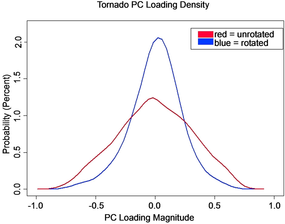
Figure 3. Empirical PDFs for PC loading vector 1 unrotated (red) and Varimax rotated (blue).

Table 1. Kurtosis statistics for PC loading vectors of tornado, hail and wind outbreaks.
the large loadings are grouped in isolated clusters with areas on near-zero loadings between the clusters, according to the correlation structure of the data. This process of rotation and mapping makes analyzing high dimensional problems tractable and is amenable to physical interpretation.
The spatial properties of each vector in B depend on the number of rotated PC vectors retained (l). Therefore, it is critical to select the optimal number of vectors, k, that correspond to data signal and reject small-scale noise from eigenvalues k + 1 to the dimension associated with the order on R.
To accomplish that goal, the matrix A is transformed to B for a variable number of retained RPC vectors (i.e., 2 to l). Each solution, based on a different number of RPCs, yields a different set of patterns when the elements of B are mapped back to the Fibonacci grid. We require a set k < l that captures as much coherent large scale signal as possible that matches the patterns embedded within R. The one set of k PC loadings that relates best to the correlation matrix generating them is determined and the number of PCs retained is set to k.
The process, outlined in [18], and refined in [16], selects each vector in B and identifies the location or gridpoint associated with the largest absolute RPC loading. Next, the RPC loading vector is matched to the vector in R corresponding to the gridpoint identified with the maximum absolute loading. This method incorporates the logic that the solution associated with k PCs must have spatial structures that match optimally to those spatial structures in R. An additional advantage to post-processing or rotating the PCs is that there is no longer a predisposition to eigenvector degeneracy [18]. The two vectors are matched, through the congruence coefficient [16], a scalar quantity that is the uncentered correlation coefficient (or the cosine of the geometric angle between the two vectors). The congruence coefficient measures both phase and magnitude match. The values of congruence range from −1 to +1, with +1 being a perfect match. The application of the congruence coefficient in this manner provides an objective procedure to select k objectively. For the tornadic outbreak set, the Varimax solution with the optimum match occurred as k = 10 (average congruence was 0.90) associated with 51.5% of the explained variance, for the hail outbreak set the optimum match was at k = 9 (average congruence was 0.91) with 41.2% of the explained variance and for the wind data set, k = 11 (average congruence was 0.92) with 48.9% of the explained variance. Thus, among these datasets, the data compression was impressive (12.8%, 3.6% and 8.5% of the basis vectors associated with non-zero eigenvalues of tornadoes, hail and wind outbreaks accounted for 51.5%, 41.2% and 48.9% of the total variance, respectively).
Step 11. Once the spatial patterns have been identified, the projections of the standardized data on the loadings are calculated to obtain the amount of each RPC pattern associated with each outbreak (e.g., how much of RPC 1 exists in the outbreak 1 for tornadoes?). To accomplish this, the RPC scores (F) are calculated as
 (6)
(6)
The PC scores are in units of standard deviations from the mean.
Step 12. A physical interpretation of the standardized anomaly fields associated with each mode involves multiplying the PC score is by the PC loading [7]. For example, a negative anomaly in a RPC loading map of geopotential multiplied by a negative PC score gives the interpretation of a positive height anomaly. Interpretation of the graphical and mapped RPC loadings and time series of the RPC scores will now be presented.
3. Interpretation of RPCA of Severe Weather Outbreak Types
3.1. Scatterplot Analysis of RPC Loadings
Normally, for datasets with a small number of variables, the RPC loadings are inspected in a table and similarities noted. However, in the present analysis, there are 26,394 elements for each loading vector, making a tabular inspection of each element intractable. To assess the coherence of the loadings for such a large number of elements requires a graphical technique that plots the RPC loadings for each vector retained as a biplot or scatterplot. The goal is to investigate whether the variables cluster into coherent groups that can be interpreted when mapped back to the Fibonacci grid. Because PC (or RPC) loading values of < |0.25| are considered essentially sampling deviations from zero [19], those variables exist in a hyperplane of width ± 0.25. Interpretation of the scatterplots of the pairs of PC loadings (the first two for each outbreak type are shown in Figure 4) indicates that the Tornado Outbreaks
 (a)
(a) (b)
(b) (c)
(c)
Figure 4. Scatterplots of the leading two rotated PC loadings for tornado, hail and wind outbreaks. The hyperplane on each plot is identified as the region < |0.25|.
majority of variables exist close to the origin of the graph, within the hyperplane.
For the tornado outbreaks (Figure 4), there is a clear orientation of variables along the RPC axes in the xand y-axis directions, suggesting well-defined modes of variation as the axes represent the RPCs. In contrast, the hail outbreaks exhibit more of a “bulls-eye” pattern with the highest concentration in the hyperplane and less distinct clustering along the RPC axes (Figure 4). This configuration of variables is indicative of the lower variance explained in hail events. The wind outbreaks plot (Figure 4) has a configuration of clustering along the RPC axes, consistent with the higher amount of variance explained with fewer PCs retained. Overall, Figure 4 demonstrates that modes of variation have clusters of variables that can be investigated further in spatial analyses of the RPC loadings plotted on the Fibonacci grids and the associated time series graphics.
3.2. Interpretation of the RPC Loading Maps for Each Outbreak Type
The outbreak RPC loadings can be interpreted when plotted to the Fibonacci grids and then isoplethed to produce fields of the variables. As there are 83 variables per outbreak type, three outbreak types with 9, 10 and 11 RPCs, that is 83 × 30 maps of PC loadings. Since the atmosphere is sampled for many variables in 3-dimensions, it is possible to examine many additional vertical slice maps. We will present just a small fraction of the results to illustrate the differences in the physical meteorological variables as a function of outbreak type. The mean sealevel pressure for the three outbreak types is shown in Figure 5. Convective storms are often linked to cyclones that are associated with relatively low pressure. Such cyclones induce low-level convergence and the associated vertical motion. It is important to note that these maps are generated for data that were collected 24 hours prior to the onset of the outbreak. Hence these are precursor fields. Additionally, the grid the data are placed on was moved to be centered on the outbreak centroid. Therefore, the “X” in Figure 5 in southeastern Kansas, meant to show the center of the outbreak is not referenced to the specific geographical location; rather, the map is provided to convey an idea of the spatial scale and configurations of the RPC loading anomalies relative to the center of the outbreak.
Tornado outbreaks (Figure 5(a)) are characterized by negative RPC loadings to the east of the outbreak and positive loadings to the west of the outbreak. Since the sign of the loadings is arbitrary, there is ambiguity in the sign of the anomalies in Figure 5 and the RPC scores must be examined for each outbreak to assign a sign to that case. For tornadic outbreak cases with positive large

Figure 5. RPC loadings of mean sea level pressure for tornado (a), hail (b) and wind outbreaks (c).
magnitude RPC scores, the physical interpretation would be anomalously high pressure to the east and anomalously low pressure to the west. Conversely, for cases with large negative RPC scores, the interpretation would be anomalously high pressure to the east and anomalously low pressure to the west. Twenty-four hours prior to the tornado outbreaks, the center of the outbreak is on a zero line between the two anomalies. In contrast, for hail outbreaks (Figure 5(b)), there is a tripole pattern of sea-level pressure anomalies, with positive loadings close to the outbreak center and negative anomalies about 1500 km to the east and also negative anomalies to the west northwest of the outbreak centroid. Assignment of the pressure anomalies would require the same process as before: investigating the RPC scores for outbreaks of hail for a large magnitude positive or negative sign and indexing the RPC loading sign accordingly. Unlike the previous two outbreak maps, the wind outbreaks have a much weaker gradient of RPC loadings in the east-west direction (Figure 5(c)) with the center of the outbreak located in an area of weakly positive PC loadings. Recall, in the discussion of hyperplanes, any PC loading with an absolute magnitude of less than 0.25 is considered essentially zero. Therefore, the loadings to the west of the center of the outbreak correspond to near-zero anomalous pressure. Examination of the three plots in Figure 5 suggests that the sea-level pressure patterns, associated with the three outbreak types 24 hours prior to the onset of the outbreak, have different in spatial structures.
Another ingredient in severe weather outbreaks is the availability of moisture for convection. The measure of moisture used in this study is specific humidity at the 850 hPa level and is shown for the three outbreak types in Figure 6. As was the case for the sea-level pressure, these moisture data were collected 24 hours prior to the onset of the outbreak. Unlike the pressure fields, the moisture fields have a more common pattern with smaller differences in the patterns for outbreak types. For tornado outbreaks (Figure 6(a)) the RPC pattern has a negative anomaly to the southwest of the outbreak centroid, indicative of drier than average air in that location. Since the sign of the loadings is arbitrary, the sign of the anomalies requires inspecting the RPC score for any given outbreak. If that score has a large positive value, the pattern on the map is likely to be found. Alternately, for cases with large negative RPC scores, the interpretation would be anomalously moist region to the southwest of the outbreak. The leading RPC specific humidity pattern associated with hail outbreaks (Figure 6(b)) indicates a spatially extensive anomaly centered to the east northeast of the outbreak center with a strong PC loading gradient over the outbreak area. The wind outbreak RPC of specific humidity (Figure 6(c)) has a spatially extensive anomaly of loadings centered to the east of the outbreak centroid. The difference between the hail and wind outbreak patterns is the lack of a strong gradient in the latter. The third field being investigated is air temperature at 850 hPa (Figure 7). Since 850 hPa is situated relatively low in the troposphere, it gives an indication of low-level thermal properties. The change in the pattern over time is considered important for assessing the instability of the atmosphere. As for the previous two fields, these temperature data were collected 24 hours prior to the onset of the outbreak. The leading RPC loadings for the temperature field taken from the tornado outbreaks (Figure 7(a)) has a negative anomaly to the south of the outbreak centroid, indicative of cooler than average air in that location. Additionally, about 1500 km to the west of the outbreak center, there is a region of positive RPC loadings, indi-

Figure 6. RPC loadings of 850 hPa specific humidity for tornado (a), hail (b) and wind outbreaks (c).
cative of anomalously warm air. As before, since the sign of the loadings is arbitrary, the sign of the anomalies requires inspecting the RPC score for any given outbreak. If that score has a large positive value, the pattern on the map is likely to be found. Alternately, for cases with large negative RPC scores, the interpretation would be anomalously warm region to the south of the outbreak and a cool anomaly to the west. The leading RPC 850 hPa temperature pattern associated with hail outbreaks (Figure 7(b)) and wind outbreaks (Figure 7(c)) have similar patterns, with a region of negative RPC loadings to the east of the outbreak region. This would indicate a spatially extensive anomaly of cold air if the RPC scores were positive.

Figure 7. RPC loadings of 850 hPa temperatures for tornado (a), hail (b) and wind outbreaks (c).
3.3. Interpretation of RPC Score Time Series for Each Outbreak Type
Because this is a multi-field PCA, the RPC scores average all the fields in (6) with equal weight to generate standardized scores; fields with fewer levels, such as the surface variables will be represented less than those fields with 17 levels. Typically, examining the extreme positive (scores ≥ 1) and negative values (scores ≤ −1) and then identifying the outbreak cases that correspond to the extreme values facilitate interpretation of the RPC scores. The tornado outbreak RPC 1 score plot (Figure 8) indicates there are multiple outbreaks that have patterns similar to the RPC 1 loadings. The first RPC score classifies 12 (of the 79) cases (15.2%) as having spatial configurations of the standardized anomaly patterns of the variables similar to the maps shows in Figures 5-7. Only 3 of the outbreaks occurred with the spatial patterns of opposite signs to those shown in the aforementioned figures.
As suggested by the lower degree of clustering for the scatterplots of PC loadings for hail (Figure 4(b)), the hail outbreak RPC 1 score plot (Figure 9) reveals a more variable pattern compared to the tornado outbreaks. The hail outbreak scores have 41 cases (16.7%) with scores greater than or equal to 1 and 16 cases (6.5%) with scores less than or equal to −1. There is evidence in the meteorological literature that hail events can occur with varied atmospheric patterns [20]. The events with extreme scores can have their standardized anomalies compared to the spatial patterns in Figures 5-7.
The wind outbreak RPC 1 score plot (Figure 10) shows that most of the extreme score cases (29% or 22.1%) had values less than or equal to −1 and only 3 cases (2.3%) had scores greater than of equal to 1. As the majority of

Figure 8. RPC scores for the 79 tornado outbreaks.

Figure 9. RPC scores for the 245 hail outbreak cases.

Figure 10. RPC scores for the 131 wind outbreak cases.
the scores are negative, the patterns shown for the loadings (Figures 5-7) should have the signs multiplied by −1 for proper interpretation of those cases associated with the negative scores.
4. Conclusions
As observation systems generate increasingly dense datasets in space and time, the spatial correlations of the fields can be characterized by the efficient data compression provided by principal component analysis. Until recently, computational power was insufficient to diagonalize the massive data sets of the three-dimensional atmosphere, as currently they are of order 108 - 109 elements and will increase further to 1010 elements and greater in the near future. The exception has been in situations where the number of cases was relatively small and the analyst was interested in time domain decomposition. We have shown that eigenanalysis of tens of thousands of variables is now achievable. The data reduction achieved in the present analyses diagonalize correlation matrices of order 26,394 dimensions and retain approximately 10 principal components for close to 50% of the variability explained. These principal components are rotated to find the localized coherent variance structures in the data. The RPCs are related to standardized anomalies of the meteorological fields analyzed. Our analyses of the RPC loadings and scores indicate these graphical displays are useful to interpret large datasets in an efficient manner. The results of the rotated PCs for defined outbreak types build upon our previous research [9-12] by indicating that the atmospheric variables investigated exhibit different spatial configurations for each outbreak type.
The challenge is how to use the output of such analyses to improve forecasting of severe weather events. By examining fields of key meteorological variables at lead times (e.g., 24 hours) sufficient to allow for societal response prior to these outbreaks, we have created a potentially useful product. The next step is to devise a pattern recognition system that compares model predictions of the atmosphere to the patterns produced in this work.
5. Acknowledgements
All of the authors involved in this research were supported in part by the National Science Foundation Grant AGS 0831359.