Development of Safety Factors for the UT Data Analysis Method in Plant Piping ()
1. Introduction
Korea is operating 23 nuclear power plants at present, and seven more units either operational, under construction and/or in preparation stage within 10 years. A nuclear power plant is composed of numerous devices and equipment connected each other by piping components. Generally, the piping installed at the secondary system in nuclear power plants is made of carbon steel. The carbon steel components experience wall thinning as the plant operates over the years due to variety of degradation mechanisms. Under the severe water-chemical conditions of high temperature and high pressure, the components are susceptible to FAC (Flow-Accelerated Corrosion). FAC is the major cause of the inside metal loss of piping components. There is a need to continuously monitor the wall thickness of the FAC susceptible ones [1].
The utilities implement thickness inspection by UT (Ultrasonic Test) at every RFO to find wall-thinned components and, if when necessary, replace significantly worn-out ones. UT is the most widely used method among variety of non-destructive techniques for inspecting components in nuclear power plants. From the surface of components, UT can measure the components’ internal volume. Especially, in light of the radiation safety, UT does not contaminate inspectors and surroundings. However, in spite of those advantages when inspecting components, considerations must be given to the manufacturing errors, the measurement errors, the local wall thickness imbalance, the internal counterbore, the surface non-uniformity by rust or paint, and the physical size of UT transducers. Excessive high or low thickness values than surroundings by certain causes may lead to large or small wear assessments.
Utilities in Korea evaluate components’ wear using the method suggested by EPRI (Electric Power Research Institute in USA). The method determines the representative wear of inspected ones considering the greatest difference between the maximum and the minimum values of the measured data. Excessive high or low thickness data than surroundings due to certain errors possibly create undesirable effects on wear assessment [2,3].
In the previous studies [4], SAM (Square Average Method) is presented in order to judge whether the measured raw data are acceptable or not for those who measure and evaluate a large number of data in a limited time. Data are compared with the surrounding data for all the measuring points of components being inspected. SAM is designed to help increase the quality of the inspection measurements. If there are any unexpected high or low data in local area, re-inspections can be recommended for such points.
In general, the manner of fabrication is different by the components’ types. Depending on the manner of component manufacturing, different safety factors should be applied when reviewing the measured raw data.
In this paper, components being measured in a nuclear power plants are classified into four groups. Suitable safety factors are presented by a statistical method for each group. The factors are available for the fast judgment whether the measured raw data sets are reasonable or not.
2. Evaluation of UT Data in Nuclear Power Plants
2.1. UT Measurement of Components in Nuclear Power Plants
Utilities conduct UT measurements for more than 200 components in every refuel outage. As shown in Figure 1, UT thickness data are obtained on the intersection points of circumferential and longitudinal lines around a component surface. The measured UT data sets are managed in the form of a text file as shown in Figure 2. The data sets are imported to CHECWORKS [1]. CHECWORKS is one of FAC managing programs developed by EPRI. The program calculates wear rate and residual life of components being inspected.
2.2. UT Data Evaluation Methods
For UT data evaluation, there are two kinds of approaches. For single inspection data, Moving Blanket Method and Band Method are available. Moving Blanket Method works properly on evaluation elbow type components whose extrados thickness is typically manufactured thinner than those intrados thickness, while Band Method works suitable for evaluation straight pipe type components [5,6].
Figure 3 shows a schematic diagram of Moving Blanket Method. The blanket is placed on a certain region of the component. Then thickness variations between the maximum and the minimum data in the blanket are calculated. Same process is carried out over the full surface of the component. The maximum variation value from all blankets of the component is regarded as wear [7].
Figure 4 shows a schematic diagram of Band Method. The band is placed around circumferential direction of
the component. Then thickness variations between the maximum and the minimum data are calculated. Same process is carried out over the full surface of the component. The maximum variation value from all bends of the component is regarded as wear [7].
For multiple inspection data, Point-to-Point (PTP) method is available for wear assessments. The amount of wall thinning that has occurred between two inspections periods can be calculated by the method. The method is based on the two readings in a given grid location taken at the same physical location on the component. A difference in thickness readings at each of the grid locations is obtained. Wear at each grid location is the thickness taken at the later inspection minus the thickness taken at the earlier inspection. The largest of the grid wears is the component wear between the two outages [2,8].
2.3. Influence of UT Reading Error
The CHECWORKS is a computer program developed by EPRI to help utilities control FAC. The program evaluates wall loss of inspected components based on the method as reviewed. The assessments are used to determine the re-inspection intervals or replacement of inspected ones.
However, excessive high wear is often found because CHECWORKS is too conservative. The unreasonable wear is due to the fact that CHECWORKS does not consider measurement errors. By the same token, thickness variations after the components manufacture can be possibly considered as wear.
Table 1 shows an example of a measurement data set. Evaluations were performed by Band Method. The wear of the component is calculated as 1.093 inches based on the measured value 0.313 inches, placed on D7.
However, it is found out that 0.313 inches on D7 was influenced by measurement error. The point D7 was reinspected and the value of the point was 1.301 inches. If the re-measurement was not performed, the component would still be judged that severe wall thinning has been occurring. If the error is not to be screened out in this step, the error will significantly work in the next wear assessments. Table 2 shows the comparison of evaluation results.
3. Method of UT Reliability Analysis
3.1. Square Average Method
SAM was suggested as a method for the determination whether the raw data are acceptable or not. The method is based on comparisons between a certain thickness data and the averaged data of surroundings’ thicknesses. Typically, along its length, components’ thickness is fairly uniform, slightly increasing, or decreasing. SAM is developed on the basis of two important findings drawn from wall thinning management experiences over the years. From the experience, only small area of components is not extremely thicker or thinner than the surroundings during fabrication. Also, wall-thinning induced by FAC does not occur in small areas unlike erosion.
The previous studies support that SAM can be used for the determination whether raw data are acceptable or not [4]. Figure 5 is a schematic diagram of the SAM assessment. Equation (1) is a mathematical expression of the SAM. “Not Acceptable” is determined, if the data on a certain point are greater than the safety factor’s multiple averaged value of the surrounding. Same process is performed for the entire measured points on components being inspected.
 (1)
(1)
where, SF: Safety Factor;
i, j: Grid Coordinate;
x: Thickness Reading.

Table 1. Example of band method ([unit: in]).

Table 2. Influence of UT measurement error.

Figure 5. Scheme of square average method.
SAM is designed to help increase the quality of the inspection measurements and help those who measure and evaluate a large number of data in a limited time. When “Not acceptable” data points are found based on results of SAM, re-inspections can be recommended for the points.
3.2. Analysis Method for Safety Factor
When SAM examines the measured data set, reasonable safety factors should be placed in Equation (1) considering the components’ thickness variations since manufactured.
Equation (2) is drawn to look for suitable safety factors taking into account the inspected components’ types. Equation (2) calculates x* which is a ratio of a certain point data x(i, j) and averaged value of the eight neighboring points of x(i, j). The ratio tends to be 1 in case the thickness is relatively constant, linearly increasing, or linearly decreasing. Statistical analysis is performed based on the value of x*.
 (2)
(2)
It is assumed that the results are likely to have relative frequency distributions closely resembling the bell-shape curve known as the normal distribution. The curve is centered at the mean value μ and its spread is measured by the variance σ2. The normal distribution function f(x) is given by Equation (3) [9].
 (3)
(3)
According to the previous research, repeated tests on a corroded pipe have found measurement differences in the range of ±5% of the measured wall thickness [3]. It is assumed that the comparison between the center value and the average of surrounding values is strongly related to the measurement differences of measured thickness, and thus the measured difference of ±5% is adopted as a critical value of the statistical study.
4. Safety Factor for Square Average Method
By and large, the manner of fabrication differs from the components’ types. When SAM method is applied to verifying the measured data set, suitable safety factors should be placed in Equation (1) considering the components thickness variations after manufacture. This section presents reasonable safety factors by components’ type. Statistical methods are used for finding safety factors based on numerous UT measurements.
4.1. Samples of UT Reliability Analysis
A total of 1007 components in nuclear power plants are analyzed. Each component is composed of as many as 100 to 300 measurement points. Overall, approximately 200,000 measurement data are analyzed.
Figure 6 shows a number of components by pipe size. UT measurements are performed by range from 1 to 47.5 inches. Out of 158 samples in total, 6 inch pipe is the one which has undergone the most in terms of the number of measurements.
UT measurements are performed for 9 different typeset components. Those are B (Bend), C (Counterbore), E (Elbow), L (Lateral), P (Pipe), R (Reducer), T (Tee), X (Expander), and Y (Weldolet). Elbow type, being a total of 444 components, is the most measured components. Figure 7 shows the number of components by the type.
4.2. Grouping by Components Type for Safety Factors
Components are classified into four groups considering the manner of fabrication. A total of 1,007 components are divided into four groups according to the classification criteria below. Group 1 is elbow type components that have commonly non-uniform thickness. The intrados area is typically thicker than the extrados area. Group 2 is expander/reducer type components that have different end. One side is large end while the other side is small end. Group 3 is pipe type components that have relatively uniform wall thickness. Group 4 is tee/lateral type components that have branch section. Flow can be merged or separated in the intersection area.
4.2.1. Elbow Type
A total of 67,318 data points are analyzed. The average value is 1.000772, and the standard deviation is 0.019529.
Table 3 shows the statistics of elbow type samples. Figure 8 illustrates the normal distribution curve. According to statistics of elbow samples, the probability of range 0.95 < x* < 1.05 is 0.9895 in this case. This means that there is a 98.95% data acquiring chance in the range of 0.95 to 1.05 on the x*. It is reasonably acceptable according to the experiences of UT measurement.
4.2.2. Expander/Reducer Type
For expander/reducer type components, one side is large end while the other side is small end. Due to the manner of fabrication, the components are likely to have typically consistent wall thickness around the circumferential direction, but the thickness is likely to vary along the longitudinal direction.
The total number of the expander/reducer samples is 7015. Table 4 shows the statistics of expander/reducer type samples. Figure 9 illustrates the normal distribution curve of expander/reducer type samples.
According to statistics of expander/reducer type samples, the probability of 0.95 < x* < 1.05 is 0.9935 in this case. The result means that there is a 99.35% data acquiring chance in the range of 0.95 to 1.05 on the x*. It is reasonably acceptable according to the experiences of UT measurement.

Table 3. Statistics of elbow type samples.

Figure 8. Normal distribution curve of elbow type.

Table 4. Statistics of expander/reducer type samples.

Figure 9. Normal distribution curve of expander/reducer type.
4.2.3. Pipe Type
A total of 17,369 data points are analyzed. Table 5 shows the statistics of pipe type samples. Figure 10 illustrates the normal distribution of pipe type samples.
According to statistics of pipe type samples, the probability of 0.95 < x* < 1.05 is 0.9942 in this case. The result shows that there is a 99.42% data acquiring chance in the range of 0.95 to 1.05 on the x*. It is reasonably acceptable according to the experiences of UT measurement.
4.2.4. Tee/Lateral Type
Tee/lateral type components are used for flow to be merged or separated. The components have a main pipe and a branch pipe. The intersection area where a branch pipe joins a main pipe is typically fabricated thicker than the adjacent area.
A total of 4818 data points are used for the analysis. Table 6 shows the statistics of tee/lateral type samples. Figure 11 illustrates the normal distribution curve of tee/ lateral type samples.
The probability of 0.95 < x* < 1.05 is 0.7455 in this case. There is a 74.55% data acquiring chance in the range of 0.95 to 1.05 on the x* for this case. This value is not acceptable according to the experiences. It is revised to the 98.95% data acquiring chance which is the result of an elbow type because this value is the most conservative among 3 other types. It is found that the safety range for the tee/lateral type is 0.896 < x* < 1.118.
5. Conclusions
This paper explores UT evaluation process used in nuclear power plants. Possible problems that are encountered during the evaluation process are also addressed. It is concluded that the measurement error can result in the unreasonable evaluation results.
Taking into account the problems which measurement errors may occur, the data reliability analysis method is reviewed for the determination whether the measured raw data are acceptable or not. The method uses safety factors for the determination. Suitable safety factors are introduced considering the type of components being inspected.
A total of 1007 components are analyzed for the determination of suitable safety factors. In a manner of fabrication, all components are classified into elbow type, expander/reducer type, pipe type and tee type components. In all cases, each group of components data samples is found to follow a normal distribution.
For the analysis, two assumptions are based on the previous study [2]. The one is that the reason for the variation of the thickness data comes from measurement error. The other one is that measurement differences are

Table 5. Statistics of pipe type samples.

Figure 10. Normal distribution curve of pipe type.

Table 6. Statistics of tee type samples.

Figure 11. Normal distribution curve of tee type.
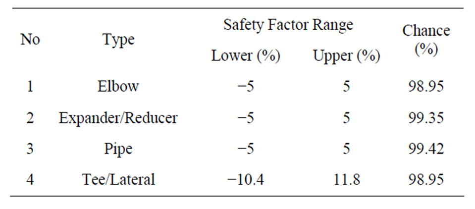
Table 7. Safety factor range of x* by components’ type.
in the range of ±5% of the measured wall thickness. Table 7 presents safety range values with the confidence level by components’ types.
The findings are expected to be useful for performing reliability analysis on the inspected data for those who measure and evaluate a large number of data in a limited time.