1. Introduction
The question of how value of firms and their debt-equity ratios are determined is a focus of debates in corporate finance, macroeconomics [2], and microeconomics [3-5]. This issue is also closely related to the determination of the cost of capital on a before and after-tax base. Moreover, in public economics research, how taxation policies affect investment and financing decisions of firms [6,7] is the acute question, which needs to be investigated because the determination of the cost of capital after taxation directly affects investment behavior of firms as well as corresponding financing decisions.
In this paper, we extend a model developed in the macroeconomics literature to analyze this problem. The model is developed under homogenous expectations in the capital market and with labor immobility within the RBC model framework, which was originally developed by [1] in relation to Tobin’s q. [4] derived the q value under monopolistic competition, and [8] derived the q value with imbedded firms’ investment functions, but we incorporate the formulation of the corporate and personal tax in a general equilibrium model as was also used in [2].
Our paper is the first general equilibrium model which extends [1] with taxation parameters and the government sector, and it addresses our original concept of “unlevered q” within this general equilibrium framework1.
In the empirical part of the paper we focus on our constructed q variable because it is the variable that can highlight firms’ real productivity. With our model, we interpret estimation results for the cost of capital and our unlevered Tobin’s q on an after-tax basis using recent Japanese data, with particular attention to the different phases of business cycles.
As to the estimation method of our constructed Tobin’s q, even though the estimation of Tobin’s q in relation to firms’ investment decisions has been conducted by [11, 12] with estimated replacement cost for Japanese data, we utilize a simplified method proposed by [13,14] as advocated by [15]. The estimation method for the cost of capital in this paper follows that of [16], utilizing asset pricing theory in the finance literature. Our sample firms are non-financial firms listed on the First and Second Sections of the Tokyo Stock Exchange. The computations of the effective marginal tax rates are conducted utilizing a simulation method proposed by [17].
Section 2 demonstrates our two-sector RBC model and presents some comparative static results. Section 3 explains our data and the estimation method. Section 4 reports our empirical result. Section 5 reaches a conclusion.
2. Two-Sector General Equilibrium Model with Taxation and Government
The theoretical relationship between production technology and asset returns is previously analyzed in [18,19] in a general equilibrium model. The Euler condition equations where both investment returns and asset returns are included are derived by [20]. In this paper, we instead use a model developed by [1] to distinguish between firm decisions in the investment goods sector and consumption goods sector for which we expect business cycle implications to be quite different2.
In the current paper, we introduce a government sector as an extra agent to collect tax and conduct infrastructure investment, in addition to the two private sectors used in [1]. The government can change tax parameters, and accordingly, equilibrium values may change. We treat this government, however, as a passive agent and do not assume any kind of maximizing behavior on the part of government in our model for the sake of simplicity. In other words, our government just equates the tax income and its infrastructure investment as if it is an identity equation3. Our model is also closely related to [21] and [22], 2000) who analyze the business cycle differences between the investment goods sector and the consumption goods sector using a power utility function with habit persistence. [16] also introduces a financial sector as a straightforward extension of [21,22] and empirically analyze the business cycle co-movements of Japanese firms in the capital market.
In an original two-sector economy model by [1], consumption goods and investment goods are produced in separate sectors. Investment goods, which we call capital goods, are resold at the end of every period and depreciable, and consumption goods are perishable. The household commits her employment contract prior to realizations of the state of nature, and firms issue risk-free debt as well as equity. The household is assumed to be equipped with a log utility function with habit persistence. The original model of [1] is proven to follow the steady-state equilibrium path, and the equilibrium equity return, as a random variable, also follows the stochastic process for each production sector.
In this paper we extend their model by incorporating both the corporate tax and the individual income tax within their general equilibrium framework and also introduce the tax savings effect of utilizing firms’ debt, which is nothing but the subsidy by the government for the use of corporate debt. The question is whether that subsidy enhances a firm’s productivity or is detrimental to it. An answer to this question can be given by utilizing our new concept of the unlevered q.
Our model specification is the following. First, we write out the consumers’ problem. The preference for households is as shown in Equation (1). In Equation (1), Ct is consumption,  is a subjective discount factor
 , Xt is an evolution of habit stock whose movements are as described in Equation (2),
  are the labor hours spent in the investment goods sector and in the consumption goods sector, respectively. The habit is the minimum level of desired consumption. Note the labor work hours are standardized to one as usual. Finally, the parameter
  is a positive scalar to denote the utility derived from leisure4. As in [1] we assume that the there is pre-commitment in the household’s labor decision. Then, she decides her consumption decision as well as stock and bond holding decisions. However, as we explain below, we assume that firms announce their real investment decision and financing leverage decision plan just before the household reaches consumption and portfolio decisions. At the end of each period government collects tax and automatically invests in the infrastructure that determines the productivity technology level. Finally, the individual, firms, and the government simultaneously reach equilibrium for each. In other words, at the beginning of every period there are three staged discrete time frameworks as in a cash-inadvance model.
The expectations in (1) are taken at the end of the previous period  after the pre-committed working decision is
 , already done as in cash-in-advance models.
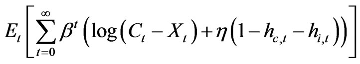 (1)
(1)
where the habit evolves following (2),
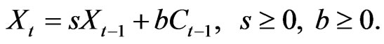 (2)
(2)
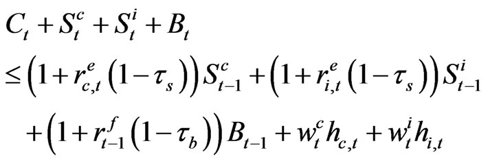
Then, the budget constraint for the household is the following. The portfolio decision is also made in conjunction with consumption decisions at the beginning of the period t but after the labor decisions are done. Note also it is done after the firm announces its investment and the leverage plan, the firm’s decision, and an individual’s decision is made simultaneously along with the government infrastructure investment.
 (3)
(3)
In Equation (3),  is the market value of equity at time t,
  is the net rate of return on equity,
  is the market value of corporate bonds,
  is the risk free bond rate, and
  is the wage rate for each sector, Furthermore, we denote the average tax rate for the dividend and capital gains as
 , the tax rate for the interest income as
 , and for future used corporate tax rate as
  5. We abstract from ordinary income tax of the household from labor wages6.
Then, the household’s first order condition with respect to the labor decision is the following (4), wherein  is the partial derivative of Equation (1) with respect to consumption where the expectation is taken with respect to time t+1 instead of t.
 (4)
(4)
The optimum portfolio decision satisfies the following Euler conditions for stocks and bonds by solving for dynamic recursive Equation (1) assuming that the household also maximizes her/his consumption and investment decision from time  on after substituting (3) into (1) for
 . By defining
  as
as  the relative price of consumption goods between time t and time
  as an optimal solution for the consumer maximization problem, we get the following:
 (5)
(5)
 (6)
(6)
The firms’ production decisions are as follows. There are two goods in an economy; i.e., perishable consumption goods and depreciable investment goods. First, the technology for producing consumption goods in period t is:
 (7)
(7)
where Ct denotes consumption goods in period t, Kc,t denotes capital for producing consumption goods at the end of period , and hc,t denotes the level of labor input in the consumption goods producing sector.
  is the technology coefficient which is an increasing function of government infrastructure investment G. The covariancestationary technology shock θt is defined as in (8) where parameter ρ lies in the interval
 .
.
 (8)
(8)
Here, random variable  is distributed as
  Second, the technology for producing new investment goods is:
 (9)
(9)
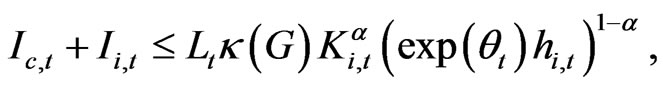
where  denote investment goods in sector
 , and hi,t denote employment in the investment goods producing sector7. In Equation (9),
  is the technology coefficient which is an increasing function of government infrastructure investment G. A logarithmic random walk technology shock Lt for this sector is defined as in (10)
 (10)
(10)
and  is distributed as
Capital stock at the end of the period is governed by the following technology:
 (11)
(11)
where y denotes the previously installed capital and z denotes new investment goods. In Equation (11),  ,
,  , and
, and .
.
Next, we introduce the tax parameter g as defined in Equation (12). Let  denote the corporate tax rate, personal average tax rate for holding stock, and personal tax rate on interest, respectively8. Then, by introducing the tax parameter g defined in Equation (12) below, we can obtain a constraint on firms’ financing decisions based on Miller’s formulation in [26]. We consider the economy before the Miller equilibrium is attained, in which the firm supply curve of the debt and the demand curve by the individual do not intersect9. This status is already verified for US firms by [27], in which he claims that the good firms do not take full advantage of government tax subsidy through the use of debt instruments because these firms want to keep their financial flexibility to prepare for financially bad times.
Thus, we define g here as
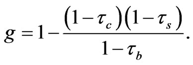 (12)
(12)
Since original stockholders receive tax shield benefits, the sum of investments on real assets and tax shields can be less than or equal to the total capital employed in the firm. The capital gains accrue to the original stockholders as an indirect subsidy from the government through a reduced corporate tax.
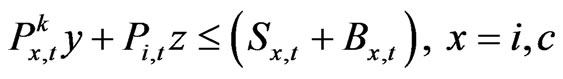
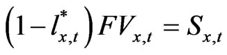
The firm’s financing constraint becomes the following inequality (13), where  is the beginning period price of the old capital,
  is the beginning period price of the new capital, Sx,t is the initial issue value of equity in industry x, and Bx,t is issued amount of risk-free debt and final term on the RHS side of the equation. The debt-tax shield accrues to the purchased stockholders and determines the next period return
  from holding the stock.
 (13)
(13)
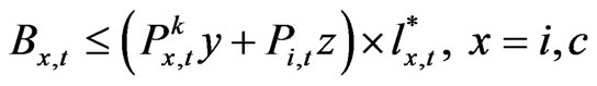
We also impose the condition that the firms set their own maximum debt amount by setting the firm target leverage ratio, partly due to flexibility reasons and partly to signaling reasons (see [16]). We denote this target leverage ratio as . This constraint is written in the following inequality (14). Because we assume that the firms have already announced the investment amount and the maximum leverage ratio at the second stage of the beginning of the period, this target will be specified by
  on the RHS of inequality (14).
 (14)
(14)
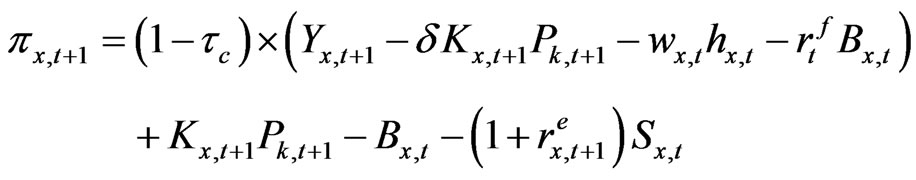
Finally, as an objective function of the firms we assume that firms choose labor and capital to maximize the profit except after payment to the bondholders of both interest and principle and to the stockholders before tax gross return from holding stock as is the case in [1]10. Note the firm in [1] is resolved every period, and firms have to pay back both the principal and interest for its debt, pay the dividend, and also buy back the stock (or liquidation dividend) before the end of the period, which becomes  in the household budget constraint (3). The profit of the firm after the corporate tax and distributions to bondholders and stockholders but before the personal tax is as follows11:
 (15)
(15)
Where  denotes a rate of return of risk-free debt and
  denotes a rate of return of an equity issued in period
  in sector x. In Equation (15) the economic depreciation rate of the capital is denoted as
  and
and  is the gross output of firms.
Then, the firm’s objective is to choose  to solve
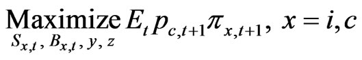 (16)
(16)
subject to constraints (13) and (14)12. The variable  is the value, measured in date
  consumption units, of a unit of date
  consumption goods indexed by state of nature and scaled by the conditional probability of that state of nature. This variable
  in (16) is defined as in the foregoing as the ratio of marginal consumption,
  in the previous Equations (5) and (6). Then, firms maximize profit after the distribution to the stockholder and the bondholder before the personal tax.
Let the marginal value to the firm of an extra unit of  be denoted by
 .
.
 (17)
(17)
Where  denotes the marginal product of capital, denoted in period
  consumption units.
Let  be the Lagrange multiplier on the financing constraint (13) and
  be the multiplier on the leverage target constraint (14). Then the Lagrange function to be maximized can be written as:
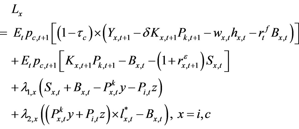 (18)
(18)
The first order optimality condition for (18) associated with  are respectively,
 (19)
(19)
 (20)
(20)
 (21)
(21)
 (22)
(22)
We can solve for these first order optimality conditions and the Euler conditions for households as well as for government revenue and the infrastructure identity Equation (28) in the following. Because the firm profit is zero and the government budget balances, it becomes the general equilibrium solution with the infinite lived household.
For this purpose let us first define the after tax bond return as  and
and  as
as
 . By first solving for Lagrange multipliers, we get the following equation for the capital goods industry13. Note also that in this case the debt-equity ratio constraint is binding14.
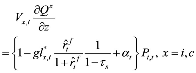 (23)
(23)
The LHS of the equation is a marginal value increase of the capital goods investment after tax for each sector, and the RHS is the price of the goods minus (inside the parenthesis) the government tax subsidy plus interest rate payments adjusted for interest rate tax.
Next, let us denote the firm value as  15. Since the relationship
 , we also get a following Equation
(24) as a value of the firm with debt.
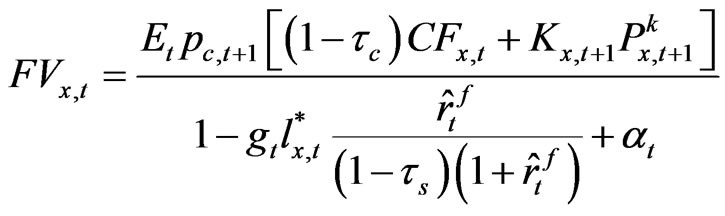 (24)
(24)
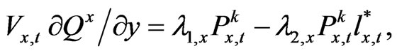
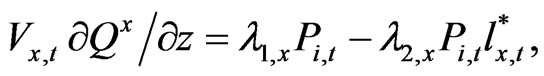
By denoting the first derivative of the  with respect to the productive capacity for the investment goods and the consumption goods as
 , we can derive the q ratio as the ratio of
  to
to . It is because the optimization condition for q is that the marginal revenue after-tax of the investment has to be equal to the q ratio, while the marginal benefit of investment is
  and the accompanying unit cost of investment is
 .
.
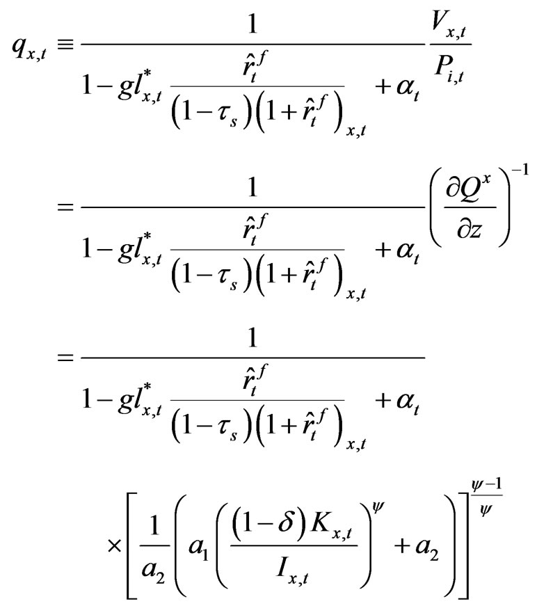 (25)
(25)
With this q value given, let us take a partial derivative of the q value with respect to the corporate tax rate and the debt ratio of the firm, respectively16.
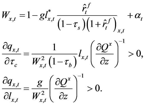 (26)
(26)
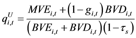
We find that our after-tax q is an increasing function of the corporate tax rate and debt ratio of the firm. The fact that q is an increasing function of the corporate tax rate may look counterintuitive because it means that raising the statutory corporate tax rate improves productivity of the firm. However, in Equation (25) note that the after-tax q-value is a product of two terms, one is , and the other is,
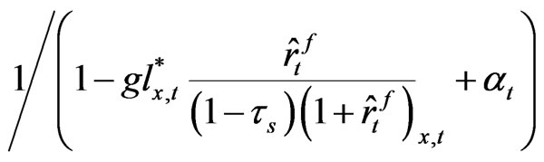 . The first term can be regarded as a q-value of an unlevered firm, and this construct, which we call “unlevered q-value”, is multiplied by the tax-shield factor
 . Obviously, we observe that the conventional Tobin’s q is a decreasing function of the corporate tax rate, contrary to the case of our unlevered q. In this paper we compute both the ordinary q-values and unlevered q-values in the empirical part and we pay particular attention to the unlevered qvalues. It is because we believe that the unlevered qvalue is a more precise measure to identify a firm’s real productivity as well as the efficiency of capital allocations.
Note up to this point the firm is assumed to maximize ex ante profit every period and the derived equations above apply only for one period. When we extend our analysis into multi-periods with infinite horizon as steady state equilibrium, we can evaluate the tax savings as a present value of the perpetual stream. When we do this, the value of the perpetual tax benefits then reduces to , and similarly the parameter
  above reduces to
  17,18.
Thus, based on Equation (23) we get the following relationship.
 (27)
(27)
Finally, by simplifying (27) we get (28).
 (28)
(28)
This equation is the final equation that bridges the conventional levered q and our unlevered q, which we will estimate in Section 4 using time-series Japanese firm data by aggregating it into the investment goods sector and the consumption goods sector.
Before we end this section, we close our model by introducing the identity equation that equates the government infrastructure investment and the tax collections from corporate income and individual financial resources. However, note in the formulation of the model that we assumed that the corporation pays for these taxes in lieu of individuals a la McGrattan and Prescott (see [2]).
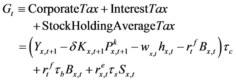 (29)
(29)
Note also that we assume  for governmental infrastructure investment.
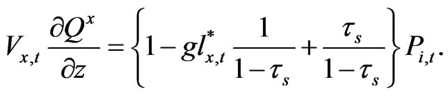
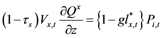
The equity rate of return formula for firms in the two production sectors in a tax-less world is given in [1,21] for a before-tax base. We extend this condition allowing for the corporate tax rate, stock holding tax rate, and the interest income withheld tax. Because the linear homogeneity of the firm’s objective, together with the inequality constraint (13), implies the equilibrium condition,  , for all
  and for all states of the nature, we get
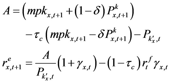 (30)
(30)
where  and
and  is the price of newly produced capital goods in sector i and sector c, for which the following (31) holds (see Appendix).
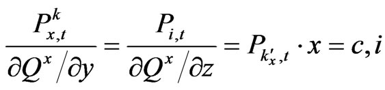 (31)
(31)
In (30) the excess return of both the investment goods sector and the consumption goods sector are functions of the capital stock and the debt-to-equity ratio of the corresponding sector, as well as various forms of tax rates. The consumption goods sector is also influenced by capital goods price changes and depreciation rates. The investment goods sector and the consumption goods sector are similarly influenced by the same capital goods price changes, while the marginal productivity of the two sectors, mpk, will be generally different among them.
These differences may cause different time patterns of the equity premium in two sectors along the different phases of the business cycles. Another parameter which produces different changes in equity premium between the two sectors is the leverage ratio of firms. Thus, the productivity parameter mpk, debt-to-equity ratio, tax rates, and the price of capital (market value of equity) all affect the rates of return on equity even before-tax as seen in Equation (30).
In Equation (30), the higher leverage causes the risk premium to be higher, as does the increase in the marginal productivity of labor and the future capital price. On one hand, higher personal taxation on capital income increases the before-tax required return. On the other hand, in our case, higher corporate tax and interest tax reduces the required rate of return19. In addition, faster economic depreciation will lead to lower required returns.
In the empirical section of the paper, we observe the time-series behavior of the required rate of return on equity and the unlevered q after-tax, and investigate how these values vary depending on historical changes in tax rates, the leverage ratios, and statutory tax rates as well as over the business cycles.
3. Data and the Estimation Method
Our data is all firms listed on the First and Second Sections of the Tokyo Stock Exchange between 1977 and 2007. The definition of each industry is from the Tokyo Stock Exchange 33 industry classifications. The definition of sectors we use is as follows. The consumption goods sector includes fisheries and agriculture, food, textiles and apparel, pharmaceuticals, electric appliances, and other products. The investment goods sector includes mining, construction, pulp and paper, chemicals, oil and coal products, rubber products, glass and ceramics products, iron and steel, nonferrous metals, metal products, machinery, transportation equipment, and precision instruments. The commerce sector includes communication, wholesale trade, retail trade, and services. The financial sector includes banks, securities, insurance, and other financial businesses. The transportation sector includes land, marine, and air transportation. Utilities include only power and gas. The real estate sector includes real estate and warehousing. The primary source for stock return data is the Nikkei Portfolio Master Data, and for financial variables we use the Nikkei NEEDS Data.
Our initial and conventional Tobin’s q estimates are computed using the simplified method proposed by [13, 14]20.
Our first Tobin’s q estimate for firm i in period t is defined as:
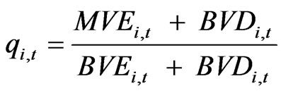 , (32)
where ,
,  and
and  denote market value of equity, book value of equity and book value of debt of firm i in period t, respectively. On the other hand, based on Equation (14) we compute unlevered Tobin’s q estimates. The approximate unlevered q is:
 . (33)
Note in the previous Equation (28) the after-tax Tobin’s q is equal to the product of unlevered q and the tax shield factor . The relation also holds between the approximate q defined in (32) and the approximate unlevered q defined in (33). One can easily check that the following (34) holds between the original Tobin’s q and our unlevered q from our stationary equilibrium solution for infinite horizons.
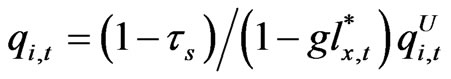 (34)
(34)
It is because the term  vanishes in equilibrium with infinite horizon time. Note that the numerator is discounted by
  in this case for infinite cash flow stream and cancel out each other on the numerator and the denominator, and furthermore one period discount rate term of the denominator does not matter in the repeated stationary equilibrium after suitably adjusting for initial boundary values.
In computing the effective marginal tax rates for each firm and for each year we adopt the definition used by [32], which is: “the present value of the current plus deferred income taxes (both explicit plus implicit) to be paid par dollar of additional (or marginal) taxable income (where taxable income is grossed up to include implicit taxes paid)21.” We employ the simulation method proposed by [17] and estimate a simple time series model of taxable income for each firm. Thus, the two tax parameters in (33),  are different across all firms and also across all fiscal years.
Here, the definition of income before-tax for our study is the sum of earnings before-tax as reported in financial statements and the net deferred tax balance divided by statutory tax rates in accordance with Japanese accounting standards22,23. The change in taxable income is defined as the change in earnings plus tax deferrals and it is assumed to follow the stochastic process (35), where  is the first difference of taxable income for firm i between the time period t and
 ,
,  the mean drift parameter for firm i, and
  an identically and independent normal random variable for all t for each i with finite and constant variance.
 (35)
(35)
The parameters of the taxable income process are estimated using the past five years of data both for the mean trend and the variance of the error term in (34) for each firm. Based on these parameter values, we then compute the expected present value of the increased tax when extra dollar (yen) income is earned by taking into account both the past five years of the tax loss carryforward benefits whenever applicable, as well as the future tax loss benefits in case firms incur losses for all 1,000 simulation paths in the future 20 years24. We use the 10 year JGB bond yield to discount the present value of tax benefits25. We also use future tax rates to compute the future tax readjustment amount by following current Japanese accounting standards26. With this method we compute the effective marginal tax rates for all firms.
4. Empirical Results
Table 1 reports the estimation results for the cost of equity for all firms listed on the First and Second Sections of the Tokyo Stock Exchange, using the version of conditional three-factor models as used in [37]. The observation period using the monthly stock return data is from September 1977 to June 2008. The detailed definition of the factor variables used is omitted, but a standard procedure is used for Fama and French three-factor model estimations, and it follows [16].
We estimate a conditional model, and for this purpose we use a natural logarithm of market size of equity and a natural logarithm of firms’ book-to-market ratio as instruments to let the sensitivity coefficient of the Fama and French three-factor model vary.
We estimate time series regression coefficients for individual stocks and take arithmetic averages for each industry as well as for two sectors used in our equilibrium model. The sector classifications are shown in the upper and lower rows of the table. We find that the cost of equity as measured in annual percent computed from the monthly data is slightly higher for the investment goods sector than for the consumption goods sector where the medians are 9.223% vs. 7.501%, and the means are 9.515% vs. 7.671%, respectively. The standard deviations are also larger for the investment goods sector with 9.795% vs. 7.671% and it implies the investment goods sector is riskier than the consumption goods sector. The size, measured by the natural logarithm of market value of equity in millions of yen, is similar between the two sectors with 10.438 vs. 10.476, and book-to-market ratios are higher for the investment goods sector at 0.725 than those for the consumption goods sector at 0.611, which means that the consumption goods sector is more of the “growth stocks” in Japan by usage in the financial economics field.
Table 2 shows summary statistics of the unlevered q which were computed using Equation (33) above. We find that the average value of the unlevered q is higher for the consumption goods sector at 1.507 than for the investment goods sector at 1.258. So is the case for the