H∞-Optimal Control for Robust Financial Asset and Input Purchasing Decisions ()
1. Introduction
When addressing any economic, finance, or engineering problem where there is uncertainty, there must be some approaches for modeling the disturbances. The use of H∞-optimal control modeling was the primary subject of control systems research in the field of engineering in the 1980s and 1990s. Many of the results of the research for continuous and discrete time systems with different information structures are presented in [1]. H∞-control, which is a minimax approach, seeks to achieve a robust design by minimizing a performance index under the worst possible disturbances, where the disturbances maximize that same performance index. In this case, robust means guaranteed performance for any disturbance sequence that satisfies the H∞-norm bound.
This is an alternative to the approaches that were primarily advanced in the 1970s. Most of that research involved the linear-quadratic-Gaussian (LQG) approach where the disturbances were treated as random and modeled with a Gaussian distribution [2,3], or with adaptive control, where the unknown disturbances are learned through feedback and feed forward loops [4]. The problem with these probabilistic approaches, such as the LQG, is that minimizing the expected value of a performance index leads to maximum system performance in the absence of misspecification, but it leads to poor performance and instability under small or large misspecifications [5]. Hence, there is a need for robust design.
In contrast to its widespread use in the engineering area, H∞-control has not been widely applied in economics and finance. One of the problems is that the system must be formulated properly with an appropriately accurate model of the system; otherwise, optimizing the wrong controller makes performance worse instead of better. Another problem with applying the H∞-approach to macroeconomic problems is that many analyses model the interdependent prices and agent’s decisions separately, so that the existing H∞-methods cannot be applied [5]. Another problem has been the modeling and computational difficulty.
There have been some economic applications, such as [6-8]. The robust method in [9] has been widely used in the area of macroeconomics. However, that method concentrates on applying entropy as a distance measure to bound uncertainty. Its examination of H∞-optimal control is limited to the frequency domain where it can be compared to the entropy approach to robust control.
The model in [5] applies the H∞-control approach to a model where agents seek robust consumption and portfolio strategies to deal with misspecifications, rather than misperceptions. He finds that H∞-forecasts are more sensitive to news than rational expectation forecasts, since robust agents behave as if they misperceive shocks to have more persistence than they actually do. The model in [5] also provides an explanation for some well-known asset pricing anomalies, including the predictability of excess returns, excess volatility, and the equity-premium puzzle. The analysis in [5] performs simulations that demonstrate that when robustness is high, prices are more volatile than dividends.
These findings add further impetus for the use of a robust approach in many areas of finance and economics. For example, it would be useful in asset and options pricing in financial markets, where common approaches, such as the Black-Scholes methodology, are sensitive to assumptions regarding the statistical distribution of the disturbances and to extreme price changes. However, [10] cautions that robust control does not imply more cautious responses than those obtained under an uncertain model. They can be more aggressive, as in the optimal monetary policy approaches of [11], or they can respond less aggressively to incoming news, as in [12].
The purpose of this paper is to model economic and financial applications using a discrete-time H∞-approach, and to develop Matlab software programs that allow users to simulate optimal solutions under a flexible choice of system parameters. The paper uses the minimax optimization approach to some fundamental economic problems where it has not previously been considered, and then compares the simulated solutions to those solutions that would have been obtained under deterministic optimal control strategies with varying parameters and terminal conditions. We develop a matrix application and a scalar application program. These programs allow the analyst to make better decisions by exploring the worstcase disturbance strategy in conjunction with other approaches to dynamic systems that contain disturbances and uncertainty.
2. Model Derivation
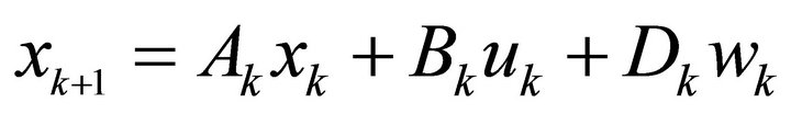
This analysis considers the discrete-time minimax controller design problem with perfect state measurements. The problem is formulated in expression (1) as a softconstrained linear-quadratic (LQ) game, which is a generalized version of that in [1]. The controller u is the minimizing player and the disturbance term w is the maximizing player.
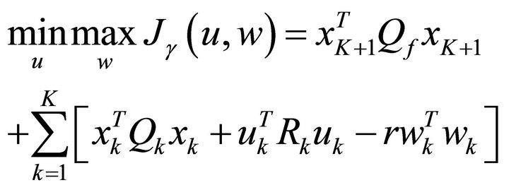 (1)
(1)
subject to
 (2)
(2)
where the initial value of the state vector at the initial time  is fixed at
 , and
, and ;
; ;
; ,
, ;
; .
.
The sizes of the matrices and vectors are as follows:
 are
are ;
;  is
is ;
;  is
is ;
;  is
is ;
;  is
is ;
;  is
is ;
;  is
is 
First, consider an open-loop information structure. As shown in [13], and later applied in [1], the game admits a unique saddle-point solution trajectory  if and only if
 ; (3)
; (3)
where , is computed by the Riccati Equation expressed in Equation (4).
 (4)
(4)
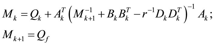
Assuming that the condition given in (3) has been met, the solution trajectory is found as follows. Define the recursive sequence of matrices  and
and , where
  is invertible, as
 ; (5)
; (5)
and
 (6)
(6)
Equations (5) and (6) can also be combined so that they can equivalently be expressed by Equation (7) as
 (7)
(7)
The unique saddle-point optimal control policy is given by
 (8)
(8)
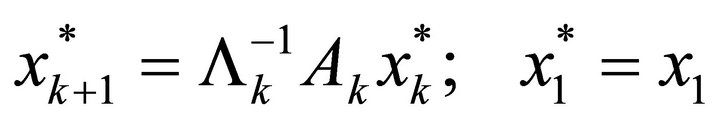
The unique saddle-point worst-case disturbance trajectory is
 (9)
(9)
and the state trajectory is
 ; (10)
The resulting saddle-point value of the game is calculated as
 (11)
(11)
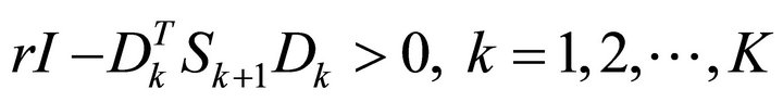
Next, consider the case where both players have access to closed-loop state information with memory. Reference [1] shows that a unique feedback saddle-point solution exists if, and only if,
 (12)
(12)
If the condition in (12) is satisfied, then the matrices , are invertible, and the unique saddle-point control, disturbance, and state trajectories are given by
 (13)
(13)
 (14)
(14)
 (15)
(15)
The saddle-point value of the game under closed-loop information is given by Equation (11), since it is the same as it was under open-loop information. If the matrix given by Equation (12) is not positive definite, and thus has one or more negative eigenvalues, then the game does not have a saddle-point solution, and its upper value is unbounded [1].
For disturbance attenuation, the value  is chosen for
 , where
 , such that
  is the infimum, i.e., the smallest value of
  that still allows for a saddle-point solution of the game. Expressions (3), (7), and (12) show that
  must be large enough to meet the conditions for the existence of a solution. Disturbance attenuation uses the minimum for
  that will satisfy these conditions. The Matlab program developed in this paper allows the user the choice to input positive values of
 , and will test to see whether the saddle-point conditions are met for the user’s chosen value of
 . Thus, the user can choose any value of
  that is large enough to satisfy these conditions, and can then choose a value that is arbitrarily close to the infimum of these values for disturbance attenuation.
Note that if the conditions in (3), (7), and (12) given above are satisfied, then the solution to the soft-constrained game defined in Equations (1) and (2) is unique and global since the game is strictly convex in u and strictly concave in w, which is proven in [1]. The computer program developed here gives the user an error message if the theorem’s conditions are not satisfied. Thus, the model will not allow the user to generate simulations in situations where the optimal (global) saddlepoint solution does not exist in the soft-constrained LQ game. The value of  must be large enough to admit a solution (if a solution exists) that will satisfy the global optimum saddle-point condition. There is no claim that this method extends to problems that are not strictly convex-concave, which cannot occur under the restricted LQ specification used in this model, given that the saddle-point solution conditions are satisfied. The global unique solution will be obtained in all cases if there is a value of the disturbance attenuation parameter that allows for a solution to the saddle-point condition matrices.
3. Application Example 1: Financial Assets
Consider a modified form of the control problem adapted from [14,15]. Suppose that an investor deposits  dollars at the beginning of year k into a bank that pays an annually compounded interest rate of
 . Let
. Let  be the account balance at the ending instant of year
 , which is the beginning instant of year k before any new deposits or withdrawals are made. The state Equation is
 (16)
(16)
Let , and assume that the initial balance in the account is zero, so that
 . Suppose that the investor’s goal is to achieve a balance of $100,000 at the end of the 10th year, i.e., the beginning of the 11th year, so that
 , and
, and .
.
One strategy would be to deposit an initial amount of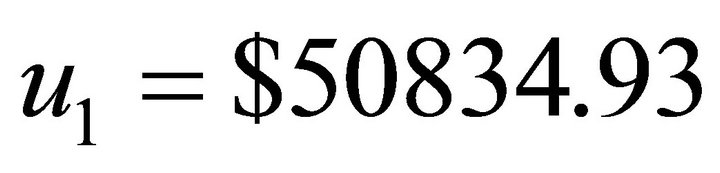 , and then let this grow to a balance of $100,000 at the end of the tenth year, as shown in Table 1. In this case, the control variable deposit amounts are
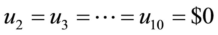 . Unfortunately, many investors would not possess the large initial deposit that would be required.
As an alternative, the investor could follow an optimal control strategy where the performance index is given by
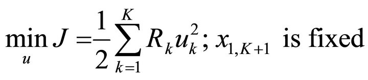 ; (17)
In this fixed terminal state case, the investor seeks to minimize the loss function in (17) subject to the state Equation
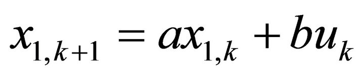 (18)
(18)
Using Equation (16), the parameters in Equation (18)

Table 1. Deterministic control with fixed final state.
are . Let the interest rate be fixed, and let the control parameter weight be fixed so that
  for all
 . The optimal control rule can be written as
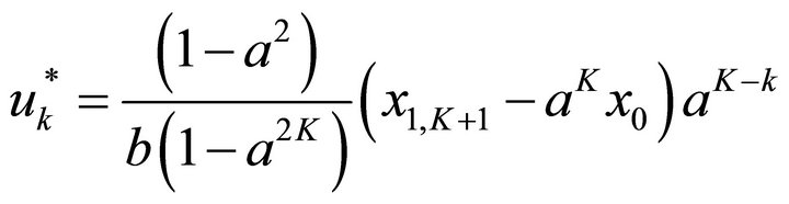 (19)
(19)
A more flexible situation would allow the investor to have a free terminal state. Suppose that the investor is interested in optimally tracking a final account balance of $100,000, but that this final value in the account at the end of the tenth year, i.e., the beginning instant of the 11th year, is variable depending on an optimal performance index. Rather than using the index in Equation (17), the investor’s objective is now to minimize the expression in (20) subject to Equation (18).
 , (20)
where  is free;
 . The solution to the optimal LQ tracking problem is given by
 (21)
(21)
where the recursive Equations are
 (22)
(22)

Table 2 shows the simulations of the tracking problem for different parameter values of , where the control weight is constant at
  for all k.
Next, consider an altered form of this problem. Suppose that an investor begins to purchase a stock, and wishes to grow the value of the portfolio to $100,000 by the ending instant of the 10th year, i.e. the beginning instant of year 11. Unlike the bank deposit, the value of the stock held in the account could increase or decrease. One option would be to model the problem as a free final state, linear-quadratic Gaussian (LQG), where the stock value fluctuations are random errors. This would provide an optimal feedback control strategy  for the stock purchase amount in each period. With perfect state information, the feedback control rule would parallel the above tracking problem, where the actual value of the account balance
  would be used in each period, rather than the deterministic, non-stochastic values in the above simulation.
Another way of obtaining insight is to consider a worst-case design approach, and formulate the problem

Table 2. Deterministic control with free final state.
through the H∞-optimal control methods discussed above. Let  be a disturbance term that represents the change in the value of the stock held in the account during period k. Let
  denote the target amount in the account at time instant k that investor is tracking, and let
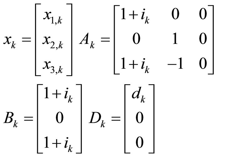
  be the difference between the actual and the desired value of the stock held in the account at time instant k. This is also a LQ tracking problem, and can be converted into a LQ regulator-type of H∞-optimal control problem by writing Equations (1) and (2) as follows:
 (23)
(23)
where, for ,
,
subject to
 (24)
(24)
where
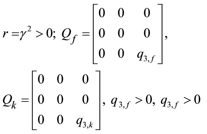
Assume that the investor starts with a zero balance and isonly concerned with getting near the final target amount of $100,000 at the final time at the end of 10 years, which is the beginning of year 11. Also assume that there is no intermediate state weighting, so that 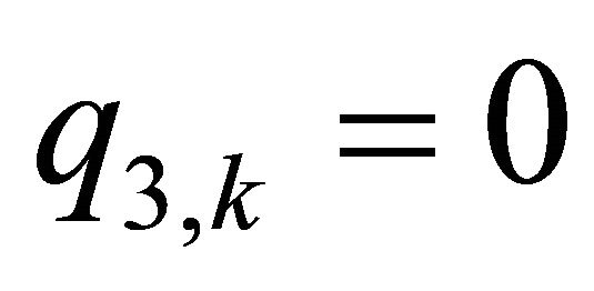 for all
 . As in the problem scenario above, assume that the long-run average rate of return is constant at
 , and that the disturbance terms represent the short-term loss in the stock value that occurs over period k, which causes the portfolio value to decline. The program allows the user to set the values for all parameters, and for the initial values in the state vector. For this example, let
  for all
 , so that the disturbance directly represents the loss in the value of the account due to the fall in the stock’s value over the period. In this case, the coefficient matrices are constant:
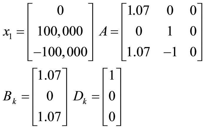
The investor is seeking to drive the shortfall in the stock account from an initial value of  to
to  at the end of the time 10-year time horizon. The more important is the goal of having a portfolio value of $100,000 at the end of 10 years, which means a reaching an account balance deficiency of
 , the higher will be the weight expressed in the parameter
 . The optimally simulated values using a closed-loop information scheme are given in Table 3.
Reference [16] uses the golden ratio as a search algorithm to compute the optimal bound for slow and fast subsystems in an H∞-suboptimal perturbation model. Reference [1] also calculates a golden ratio disturbance optimal attenuation value in a scalar model with imperfect information model where all of the performance index weights are unity, and all variables in the state and measurement Equations have unit coefficients. In order to be consistent with these previous studies, the simulations in Table 3 follow this choice of relative weighting design, and thus use , the golden ratio, as the ratio between the parameters on the final state and control

Table 3. Minimax control with higher risk exposure.
variables in the performance index. Given these parameters, the disturbance attenuation value of r = 2 is the lowest whole number value for r that admits a minimax saddle-point solution.
The results in the previous example that were shown in Table 3 can be compared to an alternative case. Suppose that the investor decides to purchase shares in mutual fund that contained both stocks and bonds, and that the mutual fund has a much lower variance, or volatility, around its expected mean growth rate. This less-risky alternative provides an intermediate case between the examples in Tables 2 and 3. Assume that the rate of return is still constant at constant at , but that
  for all
 , so that the potential loss in the value due to the disturbance is decreased. Further, assume that the final state weight in the performance index is increased from
  to
to .
.
In Table 4, the annual contributions in the  again have the decreasing pattern over time that was obtained in the deterministic case of Table 2. However, the minimax control investment strategy in Table 4 is still more aggressive and requires higher contributions than in the deterministic case. When comparing the optimal two minimax designs in Tables 3 and 4, note that the optimal control annual contributions are much higher in Table 3 when the risk exposure is greater. And, when the penalty weight on the final deviation of the state variable from its target is increased to
 , the final account balance is closer to the target amount in Table 4 than it was in Table 3.
Note that the authors have run many sensitivity simulations with various values for all of the parameters, and the performance index weights above can be chosen
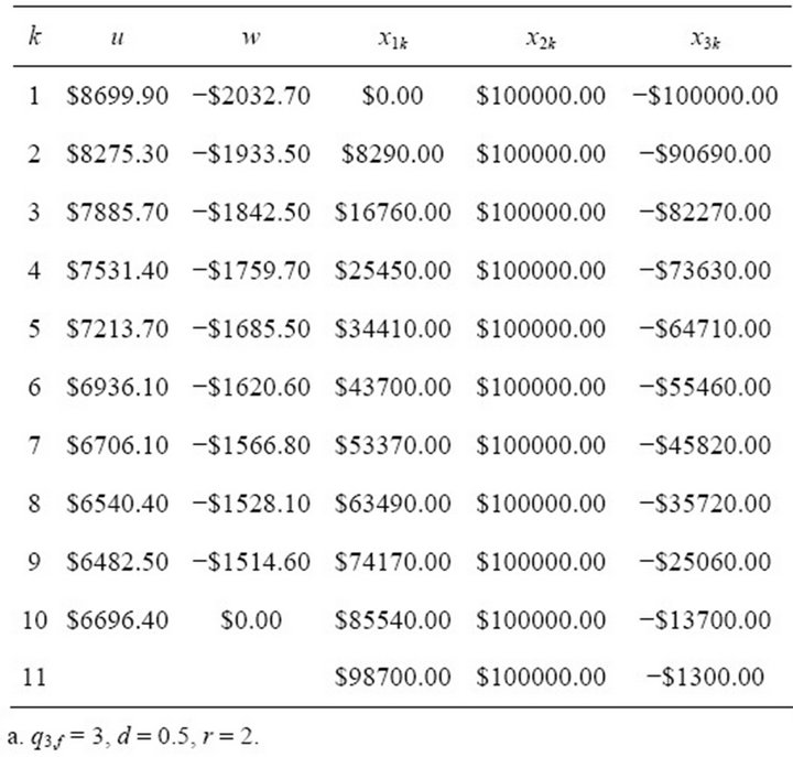
Table 4. Minimax control with lower risk exposure.
arbitrarily. The Matlab program is included in the Appendix, and users can run their own simulations. Portions of the program can be modified to handle other similar applications in economics and finance, and the authors have done this to handle other types of LQ tracking problems with higher dimensional matrices. Due to brevity and space considerations, only the simulations in Tables 3 and 4 are reported here. Comparing these results to those in Table 2 shows that the investor will optimally follow a strategy that requires a higher dollar input in each period in order to counteract the short-term disturbances when the stock or bundled portfolio underperforms its trend growth.
The minimax strategy can be employed in different ways. The investor could follow the simulated H∞-optimal control strategy when purchasing stock in each period k. Alternatively, the investor could treat the disturbance value losses as the shortfalls that need to be covered through additional deposits. These shortfalls could be added to the control inputs, i.e., the investment amounts in each respective period k, within the previous deterministic LQ-tracking problem. The investor could also design a control rule that used a weighted average of the controls, or disturbances, from standard LQ-tracker and the H∞-optimal control analysis in order compromise between the two approaches. All of these options allow the user, or investor, to evaluate and incorporate robustness considerations when formulating the feedback control investment, and to develop a desired hedge strategy.
4. Application Example 2: Input Purchasing
Consider the purchasing agent for a retail electricity supplier in a deregulated market. Wholesale electricity generation markets are generally characterized by fixedprice forward contracts, where the delivery price of some fixed quantity of electricity is determined during some period in advance of the hour of delivery, or transmission. Wholesale electricity sellers have an incentive to sign contracts in order to ensure demand, gain advantage over competitors, and deter market entry. Purchasers will sign contracts in order to reduce uncertainty over prices and quantities. Note that this analysis actually applies to any industry where inputs are commonly purchased through advanced forward contracts. This also includes electricity generator firms who are purchasing natural gas and coal inputs in the forward market to hedge against unexpected increases in input prices.
Assume that the demand for electricity for the retail utility firm has been growing at a constant average rate of i per period, so that . Also assume that the retail plant manager would like to sign forward contracts to satisfy the firm’s entire predicted demand. This can be modeled by a scalar version of Equations (1) and (2). Let
  be the control variable that denotes net change in the forward contract position from the previous period. In other words, it is the quantity of electricity (measured in megawatt hours) that the plant manager purchases in the forward market that is in addition to the previous forward purchase amount in period k under a fixed-price forward contract to be delivered in period
 . Let
. Let  be the difference between the retail demand for electricity (measured in megawatt hours) during period k, and the total amount of fix-price forward contracts that are already in place in period k. Thus, the plant manager is seeking to steer the final value of the state variable to
 . Since each quantity purchased forward reduces the residual excess demand, B will be negative. For the simulations, let B = −1, and let D = 1 since the disturbance term
  represents unanticipated excess demand.
This problem lends itself to robust considerations, since the input purchaser will face exposure to potentially high market prices during the period of high demand. In many cases, these price fluctuations will not be characterized by a stochastic error term with a constant distribution. Thus, the information gained from minimax simulation analysis would prove helpful.
Tables 5 and 6 show simulations for different parameters, where K = 12. Table 5 uses a demand growth rate of i = 0.03, and Table 5 uses a growth rate of i = 0.02. These tables use the minimum whole number disturbance attenuation values for γ that allow the saddle-point solution existence condition to be satisfied. Note that the authors have run many simulations, and are only including the following examples as illustrations. The Matlab program for this scalar system is available from the authors upon request, and can be applied toward

Table 5. Scalar simulation with smaller state weights.
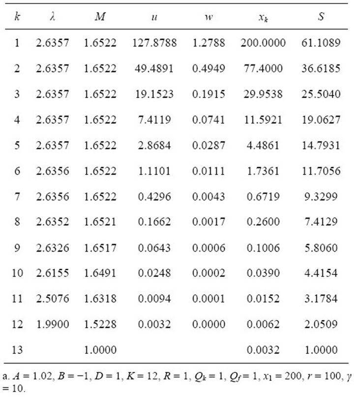
Table 6. Scalar simulation with larger state weights.
finding the H∞-optimal solution for any scalar analysis that uses expressions (1) and (2).
When the state variable parameter weights Qf and Qk are larger, the purchaser will arrange more fix-price forward contracts during the earlier periods, and the worstcase disturbance term is driven down faster. As shown in
Table 6, the purchaser will have purchased almost all of the required input in the forward market by the end of the planning horizon. As in the previous financial application example, this type of analysis can be used to plan a more robust optimal managerial strategy.