Stress and Strain Accumulation Due to a Long Dip-Slip Fault Movement in an Elastic-Layer over a Viscoelastic Half Space Model of the Lithosphere-Asthenosphere System ()
1. Introduction
It is the observational fact that while some faults are strike slip (finite or infinite in length) in nature, there are faults (e.g., Sierra Nevada/Owens valley: Basin and Range faults, Rocky Mountains, Himalayas, Atlantic fault of central Greece—a steeply dipping fault with dip 60, 80 (deg)) where the surface level changes during the motion i.e. the faults are dip-slip in nature.
A pioneering work involving static ground deformation in elastic media was initiated by [1,2]. Ref. [3] did a wonderful work in analyzing the displacement, stress and strain for dip-slip movement. Later some theoretical models in this direction have been formulated by a number of authors like [4-30]. Ref. [31] has discussed various aspects of fault movement in his book. Ref. [32] has discussed stress accumulation near buried fault in lithosphere-asthenosphere system. The work of [33] can also be mentioned in these connections.
In most of these works the medium were taken to be elastic and/or viscoelastic, but a layered model with elastic layer(s) over elastic or viscoelastic half space will be a more realistic one for lithosphere-asthenosphere system.
In the present case we consider a long dip-slip fault situated in an elastic layer over a viscoelastic half space which reaches up to the free surface. The medium is under the influence of tectonic forces due to mantle convection or some related phenomena. The fault is assumed to undergo a slipping movement when the stresses in the region exceed certain threshold values.
In our paper, we consider an elastic layer over a viscoelastic half space to represent the lithosphere-asthenosphere system, with constant rigidity (2.0 ´ 105 Mpa) and viscosity (1020 - 1021 pa∙s) following the observational data mentioned by [34,35]. Analytical expressions for displacements, stresses and strains in the system are obtained both before and after the fault movement using appropriate mathematical technique involving integral transformation and Green’s function. Numerical computational works have been carried out with suitable values of the model parameters and the nature of the stress and strain accumulation in the medium have been investigated.
2. Formulation
We consider a long dip-slip fault F and width D situated in an elastic layer over a viscoelastic half space of linear Maxwell type.
A Cartesian co-ordinate system is used with a suitable point O on the strike of the fault as the originY1 axis along the strike of the fault, Y2 axis is as shown in Figure 1 and y3 axis pointing downwards. We choose another co ordinate system ,
,  and
and  axes as shown in Figure 1 below, so that the fault is given by
 . Let q be the dip of the fault F and v1, w1 be the displacement components along y2 and y3 axes respectively for the layer and v2, w2 be that for the half-space.
 , are stress and strain, k = 1 for the layer and k = 2 for the half-space and i, j = 2, 3.

Figure 1. Section of the model by the plane y1 = 0.
2.1. For an Elastic Medium the Constitutive Equations Are Taken as
For the layer: M1
 (2.1)
(2.1)
 (2.2)
(2.2)
 (2.3)
(2.3)
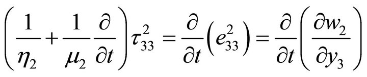
2.2. For a Viscoelastic Maxwell Type Medium the Constitutive Equations Are Taken as
For half-space: M2
 (2.4)
(2.4)
 (2.5)
(2.5)
 (2.6)
(2.6)
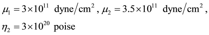
where, μ1, μ2 are the effective rigidity of the layer and the half-space respectively and h2 is the effective viscosity of the half-space.
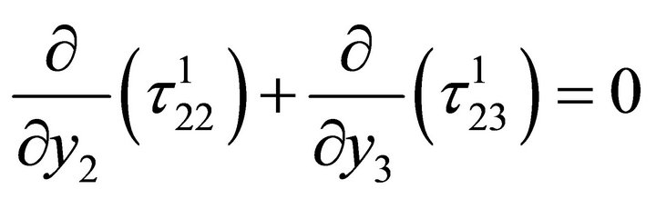
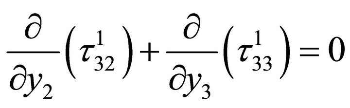
2.3. The Stresses Satisfy the Following Equations (Assuming No Changes in the External Body Force)
For M1:
 (2.7)
(2.7)
 (2.8)
(2.8)
where 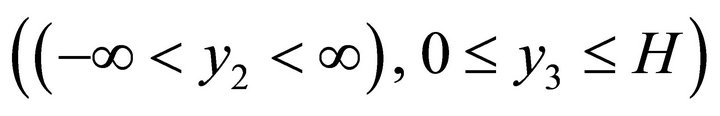
For M2:
 (2.9)
(2.9)
 (2.10)
where  and assuming quasi-static deformation for which the inertia term are neglected.
The boundary conditions are taken as, with t = 0 representing an instant when the medium is aseismic state.
 (2.11)
On the free surface y3 = 0, t > 0
 (2.12)
 (2.13)
Also as y3 →
 (2.14)
 (2.15)
 (2.16)
 (2.17)
[where  is the shear stress maintained by mantle convection and other tectonic phenomena throughout the medium].
2.4. The Initial Conditions Are
Let  and
and  be the value of (v2), (w2),
  and
and  at time t = 0 which are functions of y2, y3 and satisfy the relations (2.1)-(2.17).
a) Solutions in the absence of any fault dislocation [36,37]:
The boundary value problem given by (2.1)-(2.17), can be solved by taking Laplace transformation with respect to time “t” of all the constitutive equations and the boundary conditions. On taking the inverse Laplace transformation we get the solutions for displacement, stresses as:
For M1:


 (A)
(A)
From the above solution we find that  remain unchanged from the initial one, while
  increases linearly with time if we assume that
  to be constant. We assume that the geological conditions as well as the characteristic of the fault is such that when
  reaches some critical value, say
  the fault F undergoes a sudden slip along the dip direction.
The magnitude of the sudden slip shall satisfy the following conditions as discussed by [13].
(C1) Its value will be maximum on the free surface.
(C2) The magnitude of the slip will decrease with y3 as we move downwards and ultimately tends to zero near the lower edge of the fault.

b) Solutions after the fault movements [36,37]:
We assume that after a time T1, the stress component  (which is the main driving force for the dip-slip motion of the fault) exceeds the critical value
 , and the fault F undergoes a sudden slip along the dip direction, characterized by a dislocation across the fault given in (Appendix).
We solve the resulting boundary value problem by modified Green’s function method following [1,2,24] and correspondence principle (as shown in Appendix) and get the solution for displacements, stresses and strain as:
For M1:


or, 
where,
and

and

where,
where,
where,  (B)
(B)
3. Numerical Computations
Following [38] and recent studies on rheological behavior of crust and upper mantle by [34,35] the values of the model parameters are taken as:
D = Depth of the fault = 10 km [noting that the depth of all major earthquake faults are in between 10 - 15 km].
H = Thickness of the layer = 40 km. say (though the thickness varies from region to region of the Earth).
 .
.
 (200 bars), [post seismic observations reveal that stress released in major earthquake are of the order of 200 bars, in extreme cases it may be 400 bars]
and, 
We take the function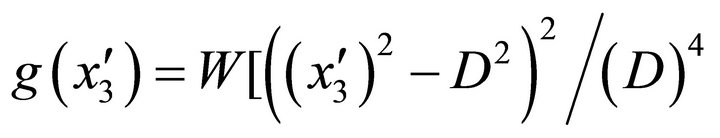 , with W = 1 cm/year, satisfying the conditions stated in
 .
.
We now compute the following quantities:
For layer M1:
 (3.1)
(3.1)
 (3.2)
(3.2)
4. Results and Discussions
The parameters involved in the expressions for displacements and stresses have been assigned appropriate values available from observed data through repeated geodetic surveys prior to and after the seismic events in seismically active regions in South and North America and China. Numerical computations are carried out using this observed values of the parameters as discussed in §3.
4.1. Variation of Vertical Component of Displacement Due to Sudden Slip across the Fault after t1 = 1 Year
“Equation (3.1)” gives us the vertical component of displacement at (y2, y3) due to the movement across the fault for different dip angle q and at different time after the fault movement. We take t1 = 1 year. In Figure 2 the graph shows the nature of surface displacement W1 against y2, the distance from the strike of the fault with q = 90 (in deg). It is observed that the displacements are in opposite directions across the strike of the fault. Their magnitudes gradually decrease and tend to zero as we move away from the fault. This is quite expected as the effect of the fault movement gradually dies out with distance. The sudden changes of W1 near y2 = 0 is due to the dip-slip motion along the fault. This is in good conformity with the result shown in Paul Segal (2010). Figure 3 shows the variation of W1 with depth y3 along the vertical through a point y2 = 5 km. for a vertical fault with q = 90 (in deg). It shows that W1 decreases sharply up to a depth of about 18 km. and thereafter diminishes to zero at a slower rate, and continuously decreases to zero for y3 > 100 km.
Figure 2. Variation of vertical component of displacement W1 with y2 for y3 = 0 km, q = 90 (deg), t1 = 1 year due to the fault movement.
Figure 3. Variation of vertical component of displacement W1 with depth y3 for y2 = 2 km, q = 90 (deg), t1 = 1 year due to the fault movement.
4.2. Variation with Depth of the Main Driving Stress t2(3( in the Dip-Slip Direction Due to the Movement across F
Figures 4-7 show the variation of  with depth y3 for various q and some specific values of y2.
In Figure 4 it is found that for a dip-slip fault with dip angle q = 30 and along the line y2 = 8 km,  undergoes a change (in one year) due to the slip movement across F. Initially there is a very small region of stressrelease just below the free surface (0 < y3 < 4.5 km). Thereafter, the rate of stress-release decreases up to a depth of 13 km and then stress begin to accumulate in the region from y3 = 13 km to y3 = 20 km after that the rate of stress accumulation gradually decreases continuously and becomes negligibly small at a depth of 50 km.
Figure 5 shows the variation of main driving stress component  with the depth of y2 = 8 km, t1 = 1 year