Hilbert Boundary Value Problem with an Unknown Function on Arbitrary Infinite Straight Line ()
1. Introduction
Various kinds of boundary value problems (BVPs) for analytic functions or polyanalytic functions have been widely investigated [1-8]. The main approach is to use the decomposition of polyanalytic functions and their generalization to transform the boundary value problems to their corresponding boundary value problems for analytic functions. Recently, inverse Riemann BVPs for generalized holomorphic functions or bianalytic functions have been investigated [9-12].
In this paper, we consider a kind of Hilbert BVP with an unknown parametric function. We first define the symmetric extension of holomorphic function about an infinite straight line passing through the origin, and discuss its several important properties. And after, we propose a Hilbert BVP with an unknown parametric function on arbitrary half-plane with its boundary passing through the origin. Then, we transform the Hilbert BVP into a Riemann BVP on the infinite straight line using the defined symmetric extension. Finally, we discuss the solvable conditions and the solution for the Hilbert BVP.
2. A Hilbert Boundary Value Problem with an Unknown Function
Let  be an infinite straight line with an inclination
  in the complex plane, passing through the origin and being oriented in upward direction. Let
  and
and  denote the upper half-plane and the lower halfplane cut by
 .
.
Our objective is to find a pair of functions 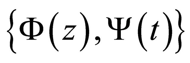 , where
  is holomorphic in the domain
  and continuously extendable to its boundary
 , and
, and  is real-valued and Holder continuous on
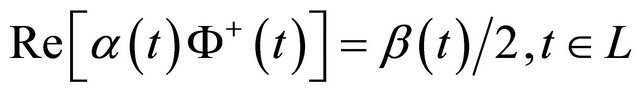
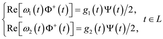
 , satisfying the following boundary conditions
 (1)
(1)
where
 and
and

are given functions.
3. Symmetric Extension of Holomorphic Functions about an Infinite Straight Line
An important step in solving problem (1) is to define a symmetric extension of holomorphic functions about the infinite straight line  with an inclination
 .
.
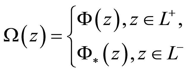
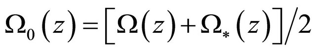
For a holomorphic function  in the simplyconnected domain
 , we define the symmetric extension of
  about
about  as follows:
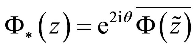 , (2)
, (2)
where  is the symmetric point of
  about
about . For simplicity, we express
  as
as . From definition (2), we may establish that 1)
 ;
;
2) If  is defined in
 , then
  is also defined in
 ;
;
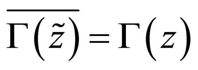
3) If  is holomorphic in
 , then
  is holomorphic in
  because of
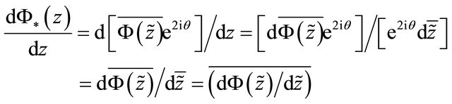 ;
;
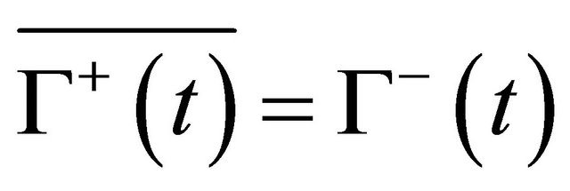
4) If a holomorphic  in
in  can be continuously extended to
 , then
  in
in  can be continuously extended to
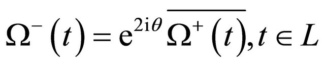
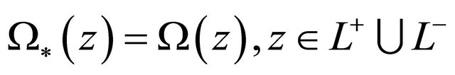
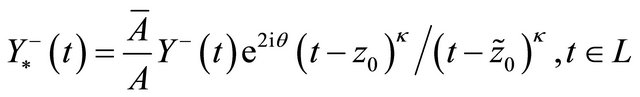
 , and their boundary value on
  satisfies the following equality
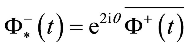 ; (3)
; (3)
5) If  is holomorphic in
  and continuous on
 , then
 (4)
(4)
is a sectionally holomorphic function that jumps on  with
with  finite, and
  possesses the following properties:
 (5)
(5)
 (6)
(6)
 (7)
(7)
6) Let , where
  and
and  are holomorphic in
  (
( or
or ). It is not necessarily true that
 .
.
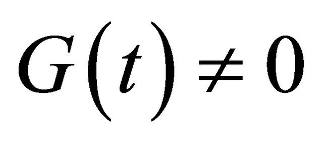
Problem (1) is normal only if  on
on .
.
4. Transformation of Problem (1)
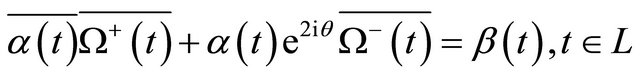
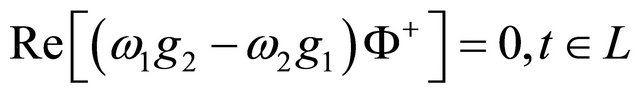
In this section, we develop a general method to solve boundary value problem (1) or similar problems. Let
Multiplying the first and the second equation in (1) by  and
and  respectively, we obtain the Riemann boundary problem
 (8)
(8)
or
 . (9)
. (9)
By extending  to
to  about the straight line
 , we obtain a sectionally holomorphic function
  as (4) with jump
 , satisfying the boundary conditions
 .
.
Thus (9) can be rewritten in the form
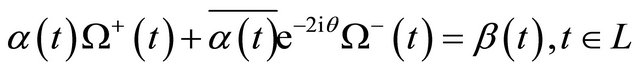 . (10)
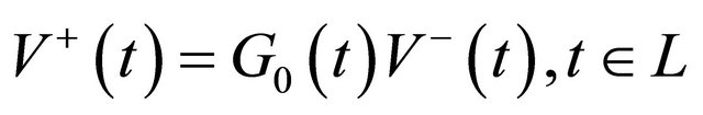
Due to , (10) can be written as R problem
 , (10)’
where
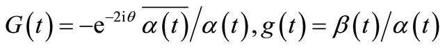 (11)
(11)
and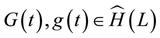 ,
, on
on .
.
If  is a solution of problem (1), then
  extended from
  by (4) must be a solution of (10) or (10)’ in
  (namely
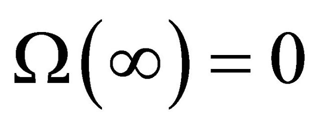 ) and satisfies the boundary condition (5). On the other hand, if the solution
  of R problem (10)’ in
  satisfies the boundary condition (5), then
 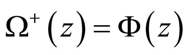 is really a solution of problem (1). Consequently, problem (1) is equivalent to R problem (10)’ in
  together with the additive condition (5).
Assume that  is a solution of (10) in
 , by making conjugate for (10) we obtain
 .
.
We read from relation (7) that  is also a solution of (10)’ in
 , so that

is a solution of (10)’ in class  and satisfies the additive condition (5). So that, whenever we find out the solution
  of problem (10)’ in class
 , and write out
 , then
is actually the solution of problem (1).
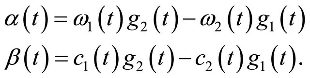
Let
 .
.
By  we know that
  is even.
5. Solution of the Hilbert Boundary Value Problem with an Unknown Function
Here, we only consider the problem (1) in the normal case. The nonnormal case can be solved similarly.
5.1. Homogeneous Problem
The homogeneous problem of (1) is as follows
 . (12)
By canceling the unknown function , problem (12) becomes
 , (13)
which corresponds to the homogeneous problem of R problem (10)’
 . (14)
Setting , we have
 .
.
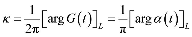
If we let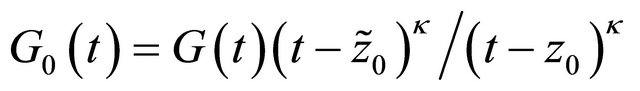 , then we know
 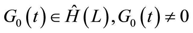 on
on  with
with
 , and
, and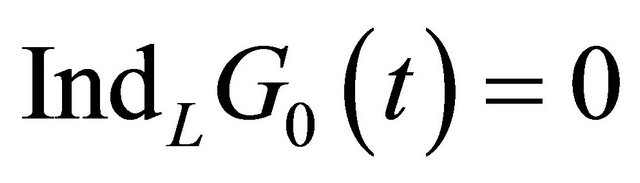 . By letting

we can rewrite (14) as follows
 . (15)
Let us introduce the function
 .
.
Since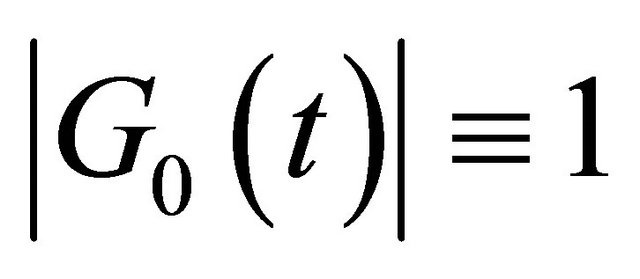 , we have
 , (16)
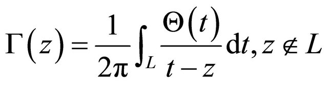
where
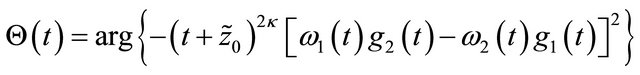
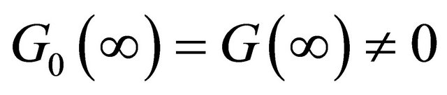
is real-valued on  and
and . Now the canonical function of R problem (15) or (14) can be taken as
 (17)
(17)
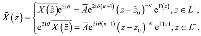
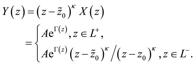
where  is an unknown complex constant. We can see from (17) that
 , thus R problem (15) can be transferred to the following problem
 . (18)
So  is holomorphic on the whole complex plane and has
  order at
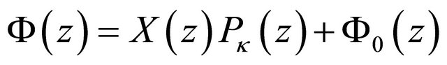
 . From [5] we know that the general solution of R problem (14) in
  takes the form
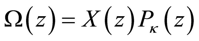 , (19)
where 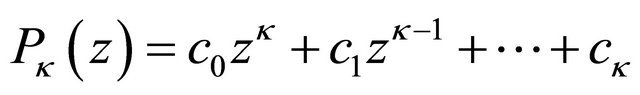 is an arbitrary polynomial of degree
  with
with  if
if .
.
According to (16), we know
 (20)
(20)
and hence
 . (21)
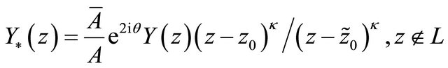
From (17) and (20) it can be seen that
which implies that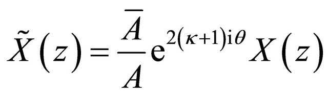 . By taking
 (22)
(22)
we obtain
 (23)
(23)
and

Consequently, we see that  if and only if
 (24)
(24)
Then when condition (24) is satisfied, the solution of H problem (13) is given by (19).
Now putting the solution  of H problem (13) given by (19) into the first equation (or the second equation) in (12), we get
 . (25)
Thus we get the following results.
Theorem 5.1. For the homogeneous problem (12), the following two cases arise.
1) When , its general solution is
 , where
  and
and  are given by (19) and (25) respectively, in which condition (24) is satisfied for
 , and
, and  is given by (22) (a real constant factor is permitted for
 ).
).
2) When , it only has zero-solution
 .
.
5.2. Nonhomogeneous Problem
In order to solve the n nonhomogeneous problem (1), we only need to find out a particular solution for problem (1).
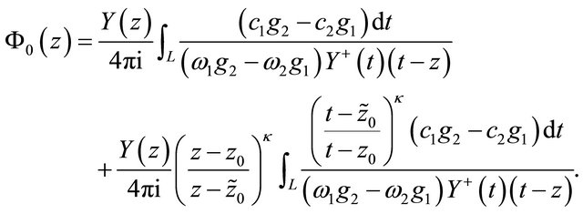
According to [5], we know that when  the R problem (10)’ a particular solution in class
  as follows
 . (26)
Therefore 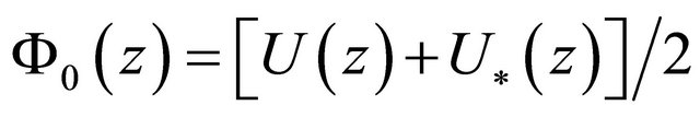 is actually the particular solution of problem (1), where
 (27)
(27)
And from (20) we obtain
 . (28)
It follows from (3) that 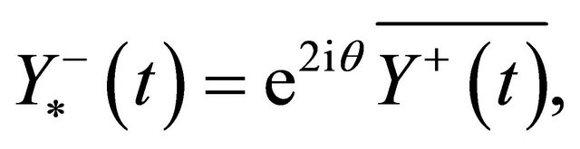 and from (20) and (21) that
 .
.
While due to 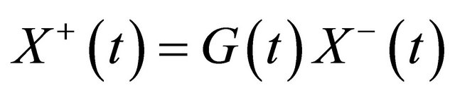 and (28) we have
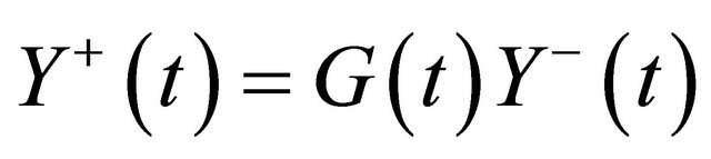 , so we obtain
 (29)
(29)
Therefore, we obtain
 (30)
(30)
and
 (31)
(31)
When ,
,  has singularity of order
  at
at . Now we aim to cancel the singularity of
  at
at . From [5], we know that R problem (10)’ is solvable in
  if and only if
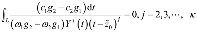 (32)
(32)
and its unique solution takes the form
 . (33)
For the case , since the solution for (10)’ in
  is unique and
  must be a solution of (10)’ in
 , we conclude that
 , thus (33) is actually the unique solution of nonhomogeneous problem (8).
Combining the particular solution of nonhomogeneous problem (8) and the general solution of homogeneous problem (14), we known that when , the general solution of R problem (8) is
 (34)
(34)
where  satisfies condition (24) and
  is given by (31); when
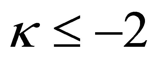 , R problem (8) is solvable if and only if (32) is satisfied and the unique solution is given by (33).
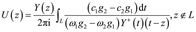
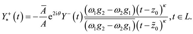
Putting the solution  into the first equation in (1), we obtain
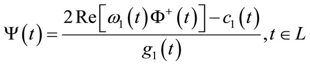 . (35)
Therefore, we derive the following results.
Theorem 5.2. If , the nonhomogeneous problem (1) is always solvable and its general solution is
 , where
  is given by (34) with
  satisfying condition (24) and
  being given by (22) (a real constant factor is permitted for
 ), while
  is given by (35). If
 , under the necessary and sufficient condition (32), the nonhomogeneous problem (1) has unique solution
 , where
  and
and  are given by (33) and (35) respectively.