1. Introduction
Let  be a probability space. The random variables we deal with are all defined on
 . Let
. Let  be a sequence of random variables. For each nonempty set
 , write
 . Given
  -algebras
  in
in , let
, let

where . Define the
  -mixing coefficients by
 (1.1)
(1.1)
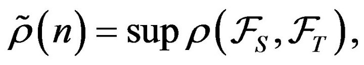
where (for a given positive integer ) this sup is taken over all pairs of nonempty finite subsets
  such that dist
 .
.
Obviously  and
and  except in the trivial case where all of the random variables
  are degenerate.
Definition 1.1. A sequence of random variables  is said to be a
  -mixing sequence of random variables if there exists
  such that
 .
.
Without loss of generality we may assume that  is such that
  (see [1]). Here we give two examples of the practical application of
  - mixing.
Example 1.1. According to the proof of Theorem 2 in [2] and Remark 3 in [1], if  is a strictly stationary Gaussian sequence which has a bounded positive spectral density
 , then the sequence
 has the property that
 . Therefore, instantaneous functions
  of such a sequence provides a class of examples for
  -mixing sequences.
Example 1.2. If  has a bounded positive spectral density
 , i.e.,
  for every t, then
 . Thus,
  is a
is a  -mixing sequence.
 -mixing is similar to
  -mixing, but both are quite different.
  is defined by (1.1) with index sets restricted to subsets S of
  and subsets
  of
of . On the other hand,
  -mixing sequence assume condition
 ,but
,but  -mixing sequence assume condition that there exists
  such that
 , from this point of view,
  -mixing is weaker than
  -mixing.
A number of writers have studied  -mixing sequences of random variables and a series of useful results have been established. We refer to [2] for the central limit theorem [1,3], for moment inequalities and the strong law of large numbers [4-9], for almost sure convergence, and [10] for maximal inequalities and the invariance principle. When these are compared with the corresponding results for sequences of independent random variables, there still remains much to be desired.
The main purpose of this paper is to study the complete convergence and weak law of large numbers of partial sums of  -mixing sequences of random variables and try to obtain some new results. We establish the complete convergence theorems and the weak law of large numbers. Our results in this paper extend and improve the corresponding results of Feller [11] and Baum and Katz [12].
Lemma 1.1. ([10], Theorem 2.1) Suppose K is a positive integer,  , and
, and . Then there exists a positive constant
  such that the following statement holds:
If  is a sequence of random variables such that
  and
and  and
and  for all
 , then for every
 ,
,

where .
.
Lemma 1.2. Let  be a
be a  -mixing sequence of random variables. Then for any
 , there exists a positive constant c such that for all
 ,
,

Proof. Let  and
and
 . Without loss of generality, assume that
 . By the Cauchy-Schwarz inequality and Lemma 1.2,

Thus

i.e.,
2. Complete Convergence
In the following, let  denote
 , and
, and 
 denote that there exists a constant
  such that
 for sufficiently large n, logx mean
 , and
, and .
.
Definition 2.1. A measurable function  is said to be a slowly varying function at
  if for any
 ,
, .
.
Lemma 2.1 ([13], Lemma 1). Let  be a slowly varying function at
 . Then i)
 .
.
ii) 
 for any
 .
.
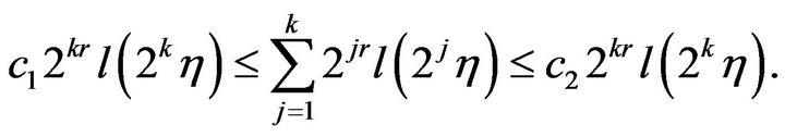
iii) For any  and
and , there exist positive constants
  and
and  (depending only on
 , and the function
 ) such that for any positive number k,
iv) For any  and
and , there exist positive constants
  and
and  (depending only on
 , and the function
 ) such that for any positive number k,

Theorem 2.1. Let  be a
be a  -mixing sequence of identically distributed random variables. Suppose that
  is a slowly varying function at
 , and also assume that for each
 , the function
  is bounded on the interval
 . Suppose
  and
and ; and if
  then suppose also that
 . Then
 (2.1)
(2.1)
and
 (2.2)
(2.2)
are equivalent.
For  we also have the following theorem under adding the condition that
  is a monotone nondecreasing function.
Theorem 2.2. Let  be a
be a  -mixing sequence of identically distributed random variables. Let
  is a slowly varying function at
  and monotone non-decreasing function. Suppose
 ; and if
  then suppose also that
 . Then
 (2.3)
(2.3)
and
 (2.4)
(2.4)
are equivalent.
Taking  and
and  respectively in Theorems 2.1 and 2.2 we can immediately obtain the following corollaries.
Corollary 2.1. Let  be a
be a  -mixing sequence of identically distributed random variables. Suppose
  and
and ; and if
  then suppose also that
 . Then
and

are equivalent.
Corollary 2.2. Let  be a
be a  -mixing sequence of identically distributed random variables. Suppose
  and
and ; and if
  then suppose also that
 . Then

and

are equivalent.
Remark 2.1. When  i.i.d., Corollary 2.5 becomes the Baum and Katz [12] complete convergence theorem. So Theorems 2.1 and 2.2 extend and improve the Baum and Katz complete convergence theorem from the i.i.d. case to
  -mixing sequences.
Remark 2.2. Letting  take various forms in Theorems 2.1 and 2.2, we can get a variety of pairs of equivalent statements, one involving a moment condition and the other involving a complete convergence condition.
Proof of Theorem 2.1. . Let
. Let
 ,
,
 . Firstly, we prove that
 (2.5)
(2.5)
By Lemma 2.1 and (2.1), it is easy to show that
 (2.6)
(2.6)
i) For , we have
 , and
, and .
.
Let  in (2.6), by
 ,
,

ii) For , let
, let  in (2.6), then
 and
and . Hence

iii) For ,
,

Noting , let
, let  in (2.6). By
 and
and , we get

By  and the Kronecker lemma,
Hence (2.5) holds. So to prove (2.2) it suffices to prove that
 (2.7)
(2.7)
and ,
,
 (2.8)
(2.8)
By Lemmas 2.1 (i), (iii), (2.1), and for each , the function
  is bounded on the interval
 ,
,
i.e., (2.7) holds.
By the Markov inequality, Lemma 1.2, Lemmas 2.1 (i), (iv), (2.1), and for each , the function
  is bounded on the interval
 ,
,

Hence, (2.8) holds.
Now we prove that (2.2)  (2.1). Obviously (2.2) implies
 (2.9)
(2.9)
Noting , by Lemma 2.1 (ii), we have

Thus,
Therefore, for sufficiently large n,

which, in conjunction with Lemma 1.2, gives

Putting this one into (2.9), we get furthermore

Thus, by Lemmas 2.1 (i), (iii),

This completes the proof of Theorem 2.1.
Proof of Theorem 2.2. (2.3)  (2.4). Let
 , the method of proof of Theorem 2.2 is similar to method used to prove the above Theorem 2.1. Only the method of prove of (2.5) is not the same. In what follows, we prove that (2.5) holds. Since
  is a monotone non-decreasing function, we have

Hence, by (2.3),
 (2.10)
i) For , by
, by  and (2.10),

ii) For , i.e.,
  ,
,

from the Kronecker lemma and

Hence (2.5) holds. The rest of the proof is similar to the corresponding part of the proof of Theorem 2.1, so we omit it.
3. Weak Law of Large Numbers
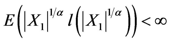
Theorem 3.1. Suppose . Let
. Let  be a
be a  -mixing sequence of identically distributed random variables satisfying
 (3.1)
(3.1)
Then
 (3.2)
(3.2)
Remark 3.1. When  and
and  i.i.d., then Theorem 3.1 is the weak law of large numbers (WLLN) due to Feller [11]. So, Theorem 3.1 extends the sufficient part of the Feller’s WLLN from the i.i.d. case to a
  -mixing setting.
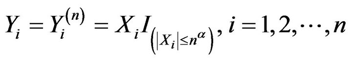
Proof of Theorem 3.1. Let  for
for  and
and . Then, for each
 ,
,
 are
are  -mixing identically distributed random variables and for every
 ,
,

via (3.1). So that (3.1) entails

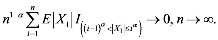
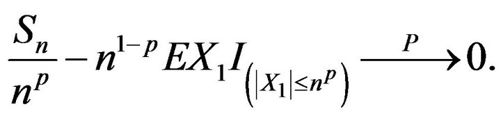
Thus, to prove (3.2) it suffices to verify that
 (3.3)
(3.3)
By (3.1) and the Toeplitz lemma,

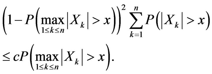
Thus, together with  for
for , we have

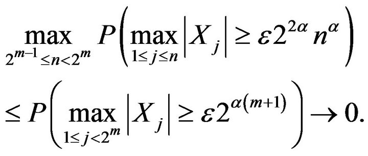
which, in conjunction with Lemma 1.1, yields for every ,
,

Thus
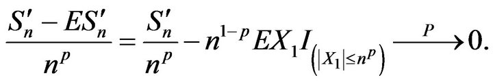
i.e. (3.3) holds.
4. Examples
In this section, we give two examples to show our Theorems.
Example 4.1. Let  be a
be a  -mixing sequence of identically distributed random variables. Suppose
  and
and ; and if
  then suppose also that
 . Assume that
  and
and  has a distribution with
 .
.
Is easy to verify that  satisfies the conditions of Theorems 2.1 and 2.2, and
 .
.
Thus, by Theorems 2.1 and 2.2,
 .
.
Example 4.2. Suppose . Let
. Let  be a
be a  -mixing sequence of identically distributed random variables. Assume that
  has a distribution with

then obviously,

Thus, by Theorem 3.1,

5. Acknowledgements
The work is supported by the National Natural Science Foundation of China (11061012), project supported by Program to Sponsor Teams for Innovation in the Construction of Talent Highlands in Guangxi Institutions of Higher Learning ([2011] 47), the Guangxi China Science Foundation (2012GXNSFAA053010), and the support program of Key Laboratory of Spatial Information and Geomatics (1103108-08).