1. Introduction
As remarked in [1], the sine-Gordon (SG) model is certainly one of the best studied of  -dimensional physics. The interest in this field theoretical model has been enhanced by its connections with the two-dimensional (2D) neutral Coulomb gas (CG) [2] and also with the 2D XY-magnetic system [3]. In this framework, it becomes an useful and powerful tool for the study of a great variety of physical properties of these two systems, which in principle admit actual realizations in nature. The SG model is also integrable in the sense that the spectrum and the S-matrix are exactly known [4,5].
In this work we employ the same methodology established in [6] in order to obtain an explicit series expression for the two-point thermal soliton correlation function in theories with a  symmetry. This has been done, firstly, by observing that when we use a polar representation for the complex scalar field in
  - dimensions described by a theory with
  symmetry, we are naturally led to a SG theory in the phase of this field [7]. Then using the connection between the SG theory and the 2D neutral CG along with the representation for the relevant soliton creation operators introduced in [8-10], and both the Euclidean thermal Green function of the 2D free massless scalar field in coordinate space and its dual [6,11], we obtain our expression for the corresponding solitonic correlation function at finite temperature.
2. Quantum Phase Solitons in Theories with a Z(N) Symmetry
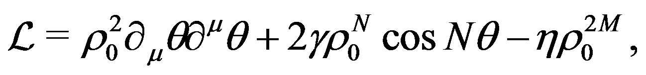
We start by considering the following theory describing a complex scalar field in  -dimensions,
 (1)
(1)
where  and
and  are integers and
  and
and  are real parameters. The above Lagrangian density is invariant under the
  transformation:
 .
.
The choice , implies the spontaneous breakdown of the
  symmetry. In this case, as is well-known, the theory will have degenerate vacua and soliton excitations. A full quantum theory of these solitons was developed in [8-10]. This includes an explicit expression for the soliton creation operator, namely
 (2)
(2)
and a general expression for its local Euclidean correlation function,
 (3)
(3)
where
 (4)
(4)
In the above expression,  is the potential of an arbitrary Lagrangian and the integral is taken along an arbitrary curve
 , connecting
  and
and . It can be shown, however, that Equation (3) is independent of the chosen curve.
We are going to show in what follows that these quantum solitons may be identified with SG quantum solitons in the phase of the field .
.
Using the polar representation for , namely,
  , where
  and
and  are real fields, we can rewrite the previous Lagrangian as
 (5)
(5)
As we shall argue, the topological properties of the theory are not affected by  fluctuations. Thus, from now on, we will make the constant
  approximation:
 (6)
(6)
Substituting the above equation into Equation (5) we obtain
 (7)
(7)
which, clearly, is a SG Lagrangian in .
.
Indeed, one may observe that the particular case of the potential appearing in the Lagrangian presented in Equation (1) for 
 (8)
(8)
presents a doubly degenerate vacuum ( symmetry), indicating the occurrence of spontaneous symmetry breaking.
After rewriting Equation (8), in terms of polar fields, as
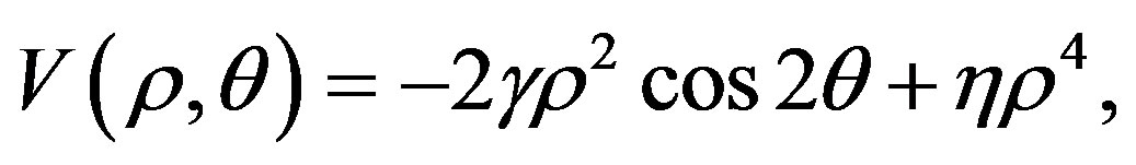 (9)
(9)
we can see that there are two degenerate minima situated at the points
 (10)
(10)
where the potential assumes the value
 . Applying, then, the constant
  approximation
 (11)
(11)
and adding  (such that the potential vanishes at its minima) we get the following SG potential for the phase field
 (12)
(12)
The above potential gives rise, when solving the corresponding Euler-Lagrange equation for the static case
 (13)
(13)
to the following solutions (classical solitonic excitations)
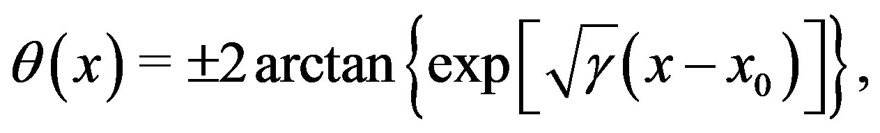 (14)
(14)
where the plus and minus signs correspond, respectively, to a soliton ( ) and an anti-soliton in the phase of the complex scalar field
 .
.
Finally, since
 (15)
(15)
we may see that this phase soliton connects the minima of the potential presented in Equation (9) when
 , as it should.
From the above considerations, we may then conclude that, in the constant- approximation, the theories given by Equation (1) will present SG solitons in the phase of the complex scalar field
 . The corresponding topological current will be
 (16)
(16)
which gives rise to the following representation for the topological charge operator
 (17)
(17)
We can see, from the above expression, that topological properties are indeed related to large  fluctuations and, therefore, the constant
  approximation should not interfere in such properties. Moreover, substituting Equation (14) into Equation (17) and making use of Equation (15), we can also see that the value of the topological charge associated to the presented classical solitonic excitations is equal to
 .
.
From a quantum mechanical point of view, however, in order to describe the quantum states associated with the classical solitonic excitations shown in Equation (14), we need to introduce a quantum soliton creation operator , whose application on the vacuum state of our theory, namely
 , yields a solitonic state
 , i.e.
  . This quantum soliton creation operator must satisfy the following commutation relation with the topological charge operator
 , presented in Equation (17):
 (18)
(18)
where  is a real constant whose meaning may be clearly understood by applying both sides of the above equation on the vacuum state
 . Indeed, since
  and
and , we have
 (19)
(19)
from which we may conclude that  is nothing but the eigenvalue of the topological charge operator
  associated to the eigenstate (solitonic state)
  or, in other words, the expectation value of
  when measured in the state
 . This property allows us to associate
  with the classical topological charge.
Thus, as we have already saw, we may explicitly confirm the fact that the soliton operators introduced in [8-10] are indeed creation operators of quantum solitons in the phase of the complex scalar field  by computing the commutation relation between the quantum soliton creation operator and the topological charge operator.
In order to do that, let us firstly observe that, since the momentum canonically conjugated to  is
is

we can rewrite the soliton creation operator for the theory described by Equation (1) in terms of polar fields (in Minkowski space) as [8-10]
 (20)
(20)
Notice that this is nothing but the Mandelstam creation operator of quantum solitons in the SG model [12], as it should. Then, using canonical commutation relations along with the well-known Baker-Campbell-Hausdorff identity , we readily find
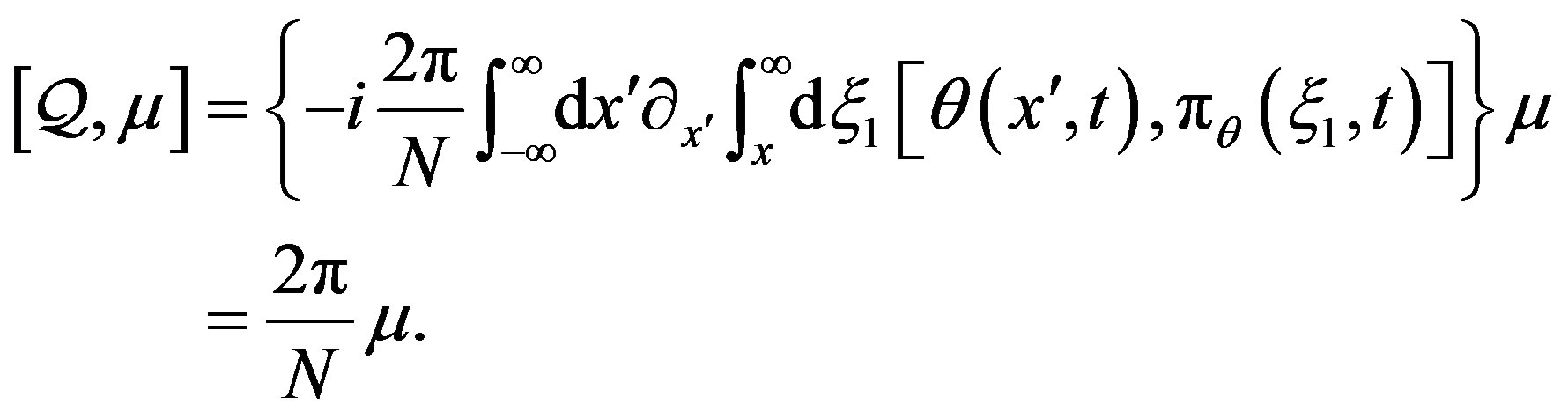 (21)
(21)
Last but not least, following the above discussion, we may notice that Equation (21) implies that the operator  creates eigenstates of the topological charge operator
  with eigenvalue
  (which, not by coincidence, for
 , corresponds to the value of the topological charge associated to the classical solitonic excitations presented in Equation (14), namely,
 ), thus proving that the quantum solitons occurring in the theory described by Equation (1) are, indeed, SG solitons in the phase of the complex scalar field
 , i.e. they are phase solitons.
In the next session, we are going to calculate the twopoint correlation function of these quantum soliton excitations at finite temperature.
3. Two-Point Thermal Soliton Correlation Function
The Euclidean vacuum functional of the SG theory, for an arbitrary  may be written as the grand-partition function of a classical 2D CG of point charges
 , contained in an infinite strip of width
 , interacting through the potential
 , namely [13]
 (22)
(22)
where ,
,  runs over all possibilities in the set
 , and
, and  is the Euclidean thermal Green function of the 2D free massless scalar theory in coordinate space
 , which is given by [14]
 (23)
(23)
with .
.
A closed-form representation for this function was presented for the first time in [15], and is given by
 (24)
(24)
This has also been obtained by using methods of integration on the complex plane [11]. At ,
,  reduces to the 2D Coulomb potential and we retrieve the usual mapping onto the Coulomb gas [2].
We may rewrite the above thermal Green function in terms of the new complex variable
 (25)
(25)
where , as
, as
 (26)
(26)
Notice that in the zero temperature limit ( ,
, ), we have
  and
and  and, therefore, we recover the well-known Green function at zero temperature, namely
 (27)
(27)
We can now determine the soliton correlation function at , by using Equation (20) along with the gas representation of the vacuum functional, Equation (22). Notice that, the insertion of
  operators corresponds, in the CG language, to the introduction of “magnetic” fluxes on the gas [8]. The soliton correlator, therefore, is nothing but the exponential of the interaction energy of the associated classical system. Charges and “magnetic” fluxes interact with their similar, through the thermal Green function
 , whereas the charge-flux interaction occurs via the dual thermal Green function
  (described in the Appendix) [8]. This is the reason why it is crucial to know this function in order to obtain the soliton correlator.
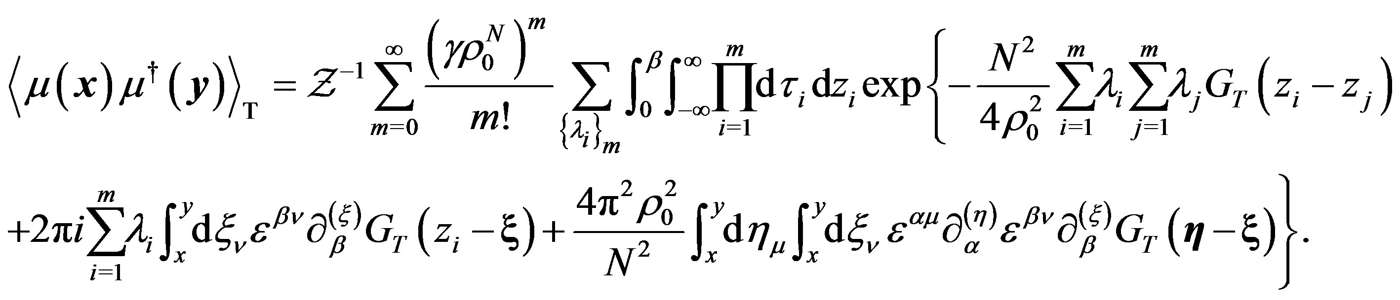
Following the above considerations and the same procedure employed at  [1], we can write the two-point thermal soliton correlation function occurring in theories with a
  symmetry as
 (28)
(28)
After some algebra, we get
 (29)
(29)
Using the Cauchy-Riemann conditions, Equation (A3), we may rewrite the above expression as
 (30)
(30)
Finally, using the UV-regulated version of , namely
 (31)
(31)
and the expression (A2) for the dual thermal Green function , we obtain
 (32)
(32)
where the renormalized coupling  (Coleman’s renormalization) is given by
[16].
Notice also that, as in the  case, existence of the
  limit imposes the neutrality of the gas, namely
 , because in this case the
  -factors are completely canceled. This implies that the index
  appearing in Equation (22) must be even (
 , with
  positive and
  negative
 ’s) and, therefore,
 .
.
Let us finally remark that in the  limit the above correlation function reduce to the corresponding function of the zero temperature theory [1], as it should.
4. Acknowledgements
This work has been supported in part by Fundação CECIERJ.
Appendix
Here we present a closed-form representation for the dual thermal Green function , which we have used for computing the soliton correlation function shown in Equation (30).
Indeed, we can see from Equation (26) that the thermal Green function may be written as the real part of an analytic function of the complex variable , namely
 (A1)
(A1)
where .
.
The imaginary part of  may be written as
 (A2)
(A2)
Now, from the analyticity of , it follows that its imaginary and real parts must satisfy the CauchyRiemann conditions, which are given by
 (A3)
(A3)
This property characterizes  as the dual thermal Green function.