Boundary Stabilization of a More General Kirchhoff-Type Beam Equation ()
1. Introduction
The problem is based on the equation

which was proposed by Woinowsky-krieger [1], as a model for vibrating beams with hinged ends. One of the first mathematical analysis for the equation

was done by Ball [2], which was later extended to an abstract setting by defining a linear operator A by Medeiros [3]. In [4], Tucsnak considered the above beam equation which clamped boundary and obtained the exponential decay of the energy when a damping of the type a(x)ut is effective near the boundary. In the same direction, Kouemon Patchen [5] obtained the exponential decay of the energy for above-equation when a nonlinear damping g(ut) was effective in Ω. To [6] considered the above kirchhoff-type beam equation under non-linear boundary conditions


which the model is clamped at x = 0 and is supported x = l. He proved the existence and decay rates of the solutions. A rather general kirchhoff-type beam equation

was set up by Ball [7], who presented the existence and uniqueness of solution under linear boundary conditions. However the global solution and exponential decay for the more general beam equation is open under nonlinear boundary conditions. In the present work, we are concerned with the existence and uniqueness of solutions and the exponential decay property of energy on the nonlinear beam equation with external load
 (1)
(1)
with nonlinear boundary conditions
 (2)
(2)
 (3)
(3)
and initial conditions
 and
and  (4)
(4)
2. Definition and Assumptions
In this paper, our analysis is based on the Sobolev spaces
 ,
,

espectively equipped with the norm  and
and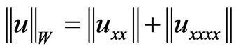 . We assume that f, g:R → R are continuously differentiable functions such that
and  (5)
(5)
where  and
and
and  (6)
(6)
for some ρ > 0.
Assume that the functions  are non-negative functions and respectively satisfy

and  (7)
(7)

and  (8)
(8)
3. Existence and Uniqueness of Global Solutions
Now we come to the following conclusions of the existence and uniqueness of global solutions.
Theorem 1. Assume that the assumptions of (5)-(8) and  hold. Then for any
  satisfying the compatibility condition
 (9)
(9)
There exists a function u satisfying (1)-(4) such that

Proof. Let us solve the variational problem associated with (1)-(4), which is given by: find  such that
 (10)
(10)
for all . Let
. Let  be a complete orthogonal system of W. For each
 , let us put
 .
.
We search for a function

where  is a unknown function such that for any
 , and it satisfies the approximating equation
 (11)
(11)
with the initial conditions
 and
and  (12)
(12)
Thus (11) and (12) are equivalent to the Cauchy problem of ODES in the variable t, which is known to have a local solution um(t) in an interval [0, tm) (tm < T) for any given T > 0.
Estimate 1. By integration of (11) over [0, t] (t < tm) with , we see that

where  and
and .
.
Considering that
 ,
,
 and the initial conditions, we get
 .
.
Using Gronwall inequality, we have . Then there exists a constant M1 depending only on T such that
 . (13)
for any  and for all
 .
.
In this paper, C is a constant independent of m, t and denotes different value in different mathematical expression.
Estimate 2. Integrating by parts (11) with  and t = 0, and considering the compatibility condition (3) we get
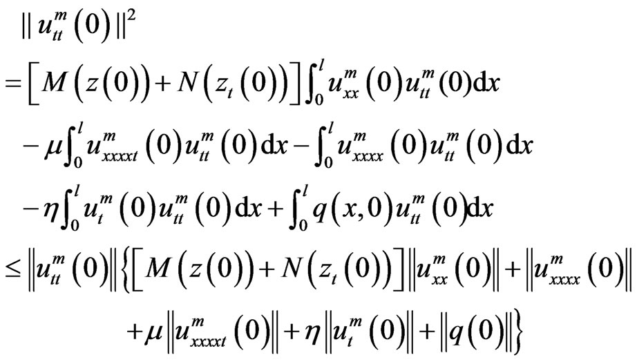
Thus there exists a positive constant M2 such that
 . (14)
Estimate 3. Let us fix t, ξ > 0 such that ξ < T – t. Taking the difference of (11) with t = t + ξ and t = t, and replacing ω by , we get

where
 .
.
Let us estimate . Since
 we have
 (16)
(16)
Noting that ΔM1 = M(z(t + ξ) – M(z(t)) and ΔM2 = N(zt(t + ξ)) – N(zt(t)), then integrating by parts we have

Since , by the Mean value theorem, from estimates 1 and (16) we have

where η1 is between  and
and .
.
By the Mean value theorem, we also have

Considering that M(z(t + ξ) ≤ C and N(z(t + ξ) ≤ C, we conclude that there exists constants k1 > 0 and k2 > 0 such that
 (17)
(17)
A argument for f yields
 (18)
(18)
where k3 > 0 is a constant. Putting

and taking into account of (17)-(18) and the assumptions of g, we deduce from (15) that
 (19)
(19)
where k4 = max{k1 + k3, k2}. Therefore
 (20)
(20)
Dividing the above inequality by ξ2 and letting ξ → 0 gives
 .
.
From estimate 2 we find a constant M3 > 0 such that
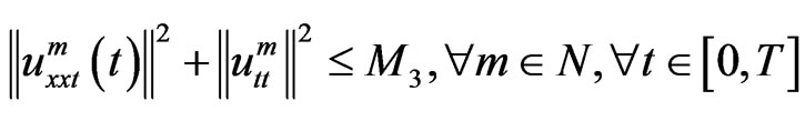 .
.
With the estimates 1 - 3 we can use Lions-Aubin Lemma to get the necessary compactness in order to pass (11) to the limit. Then it is a matter of routine to conclude the existence of the global solution in [0, T].
Theorem 2. The solution u(t) of theorem 1 is unique.
Proof. Let u, v be two solutions of (1)-(4) with the same initial data. Then writing p = u – v, putting ω = pt in (10) and using mean value theorem, chauchy-schwarz inequality and Gronwall inequality, we may get p = 0. Thus u = v.
4. The Exponential DECAY of the Energy of System
In order to establish our decay result, we define the energy of the system by

where . We have Theorem 3. Let u(t) be the solution given by theorem 1 as q(x, t) = 0 and g = 0. And assume that N(s)s ≥ 0 and f(s)s ≥ 0. Then there exist constants λ2, λ4 > 0 and λ3 < 0 such that
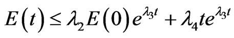 .
.
To prove Theorem 3, we firstly introduce two lemmas.
Let us define  .
.
Then we have the following lemmas.
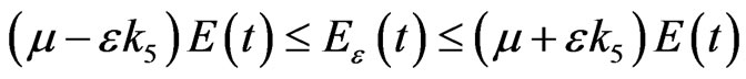
Lemma 1. Let Eε(t) = μE(t) + εψ(t). Then there exists a constant k5 > 0 such that
 .
.
Proof. By ,
,  and
and  there exists k5 > 0 such that

where .
.
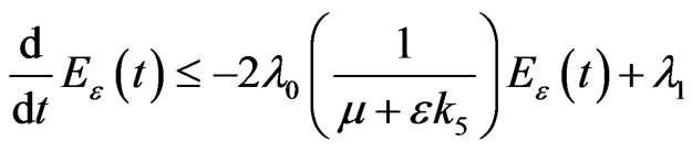
Lemma 2. There exist constants λ0 > 0 and λ1 such that
 .
.
Proof. Taking the inner product of (1) with ut and considering that N(s)s ≥ 0, we have
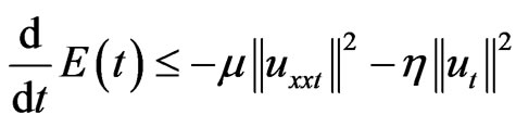 .
.
Taking the inner product of (1) with u, we have


Thus
 .
.
Set  .
.
Since , we have
 . Therefore
 .
.
From the Mean value theorem, there exists a constant λ1 such that

On writing , we have

The proof of theorem 3. From lemma 1, we have
 . (21)
From Lemma 2, we have
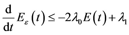 . (22)
Therefore
 .
.
By Gronwall inequality and combing (21), we have
 .
.
Hence, for sufficiently small ε > 0
 .
.
On writing 
and 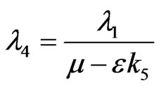 we have
  .
.
The proof of theorem 3 is now completed.
NOTES
#Corresponding author.