Impact of an External Magnetic Field on the Shear Stresses Exerted by Blood Flowing in a Large Vessel ()
1. Introduction
The aim of this paper is to provide an advanced analysis of the shear stresses exerted on vessel walls by the flowing blood, when a limb or the whole body, or a vessel prosthesis, a scaffold… is placed in an external static magnetic field B0.
As explained in [1] [2] , such a situation may occur in several biomedical applications:
・ magnetic resonance imaging (MRI) [3] [4] [5] [6] [7] .
・ magnetic drug transport and targeting [8] - [13] : magnetic particles containing or coated with therapeutics are injected into the bloodstream and concentrated to sites of disease under the influence of the magnetic field.
・ tissue engineering [14] [15] [16] [17] [18] : magneto-responsive particles are guided by the magnetic force in order to enhance cellular invasion in the scaffolds.
・ mechanotransduction studies and applications for regenerative medicine strategies (for example, with stem cells) [19] [20] .
This analysis would also provide a risk assessment for the vessel wall (plaque rupture in case of atherosclerotic lesion [21] , severity of some aneurysms [22] , ...) or for other cells attachment and/or transmigration (white blood cells, tumor cells, cells seeded in vascular substitutes [23] , ...).
Since blood is a conducting fluid, its charged particles are deviated by the Hall effect thus inducing electrical currents and voltages along the vessel walls and in the neighboring tissues. The equations of motion include the Lorentz force j^B, where j is the electric current density. Consequently, the velocity profile is no longer axisymmetric, even in a cylindrical vessel; and the velocity gradients at the wall vary all around the vessel.
To illustrate this idea, we chose to expand the exact solution given by Gold [24] for the stationary flow of blood in a rigid vessel with an insulating wall in the presence of an external static magnetic field. This analysis completes previous ones [25] [26] . In the present paper, we provide the analytical expressions for the velocity gradients and evaluate them near the vessel wall.
2. Unidirectional Steady Blood Flow in a Rigid Cylindrical Vessel with Insulating Walls
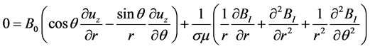
As explained by Gold [24] and by Abi-Abdallah et al. [25] , the Navier-Stokes equations including the Lorentz force (Equation (1)), coupled with the induction equation (Equation (2)) govern the flow of a conducting, incompressible, Newtonian fluid in an externally applied static magnetic field B0.
 (1)
(1)
 (2)
(2)
where u and P are the fluid velocity and pressure; μ is the magnetic permeability; ρ, η and σ are the fluid density, viscosity and conductivity and the electric current density is expressed as
.
Gold [24] then considered the case of a unidirectional steady blood flow in a rigid circular vessel with insulating walls and radius R (Figure 1, [25] [26] ). The
![]()
Figure 1. Schematic drawing of the studied problem (from [25] ). The induced currents (blue dashed lines) are oriented along (Oy) in the tube center. Since they cannot escape the vessel (insulating walls), they return adjacent to the wall. Closed loops are thus generated, and these loops induce some magnetic field BI (Biot and Savart law). This induced field is parallel to the Oz axis with opposite directions on each side of Oy.
velocity and magnetic field are defined in the cylindrical frame (er, eθ, ez) as:
 (3)
(3)
The induced magnetic field, BI, is parallel to the flow and guarantees
. The continuity equation
is also satisfied.
The longitudinal projections (along ez) of Equations ((1) and (2)) in the cylindrical frame are thus:
 (4)
(4)
 (5)
(5)
The boundary conditions associated with this problem are:
 because the wall is non-conducting (6a)
and
, because of the no-slip condition at the rigid wall (6b)
The equation system (4) to (6) is expressed in a non-dimensional form, using the following definitions:
,  ,
, and
,
, and  (where u0 is some characteristic mean velocity).
The numerical values of the different quantities are taken from Abi-Abdallah et al. [25] :
,
,
, and
; then G equals +8.
The non-dimensional solution given by Gold [24] for Equation (4) and (5), associated with the boundary conditions (6) is:
 (7)
(7)
and
(8)
with:
,
,
,
,
and
(9)
The Hartmann number, Ha, is defined as:
, the magnetic Reynolds number, Rem, as:
, and the functions In are the nth order modified Bessel functions of the first kind.
In order to evaluate the derivatives of the In functions, the following identities are used:
(10).
In such flow configuration, the classical definition of the dimensional shear stresses would yield:
(11)
The corresponding non-dimensional expressions would be:
, where
, and
(
, with the numerical data of this study).
It is thus necessary to calculate the velocity gradients (from Equation (8)). This can be done as follows:
and
(12)
(13)
(14)
and
(15)
and
(16)
Gathering all, one obtains:
(17)
and:
(18)
3. Results
The term
,
, represents the change of velocity in the radial direction, all around the vessel wall.
The term
represents the change of velocity in the azimuthal direction, at a given value of
. The velocity is zero everywhere at the wall (r = R); consequently the velocity gradient
is also zero. The interesting quantities are thus
, for
close to 1, but lower than 1.
The dependence of the non-dimensional velocity
upon θ (for
) is presented in Figure 2. It has been computed for
. In the absence of magnetic field (Ha = 0), the situation is axisymmetric and the velocity does not depend upon θ. The flow is the classical Poiseuille flow and, as expected,
. When the Hartmann number increases, the flow is furthermore reduced (this is the decelerating effect due to the Lorentz force), and the dependence upon θ (asymmetry of the flow) is more and more pronounced. The velocity is maximal in the direction θ = 0 and θ = π (or −π), according to the fact that the profile is flattened and stretched parallel to the direction of B0 (along Ox) [25] . For the same reason, the velocity is minimal in the direction θ = π/2 or −π/2.
The same type of results is shown in Figure 3, where the dependence of the velocity upon θ has been illustrated at
(near the vessel wall). Of course, the velocities are very small, since at the wall, they are exactly zero. As in Figure 2, we can observe that the curve obtained for the case Ha = 0.16 is superimposed with the curve Ha = 0, meaning that the influence of a magnetic field B0 =1.5 T (corresponding to Ha = 0.16) remains negligible. Moreover, when Ha = 0, the
![]()
Figure 2. Dependence of the non-dimensional velocity
upon θ (for
), at
.
![]()
Figure 3. Dependence of the non-dimensional velocity
upon θ (for
), at
.
![]()
Figure 4. Dependence of the non-dimensional velocity gradient
upon θ (for
), at
.
value obtained for the non-dimensional velocity at r = 0.99 * R is 0.0398, which is the Poiseuille value.
The dependence of the non-dimensional velocity gradient
upon θ (for
), at
is illustrated in Figure 4 and at
in Figure 5. These gradients are negative, since the value of the velocity
decreases when going towards the vessel wall (
, when
). As previously noted, the influence of a 1.5 T magnetic field (Ha = 0.16) is not discernible, and the absolute values of the gradients
are maximum for θ = 0, and θ = π, or −π (due to the fact that the profile is stretched along Ox).
In the absence of a magnetic field (Ha = 0), the Poiseuille value (
, at the wall) is obtained, and no dependence upon θ is observed (axisymmetric situation). The maximum values of
are increased by about 25% in the case of a very strong magnetic field (Ha = 4.47, B0 = 40 T), when compared to the case Ha = 0.
The dependence of the non-dimensional velocity gradient
upon θ (for
), at
and at
is illustrated in Figure 6 and Figure 7 respectively. Since we have
, everywhere at the vessel wall (
), we also have
, for
. Consequently, the absolute values of the
velocity gradients decrease when
tends towards 1.
In the absence of a magnetic field (Ha = 0), the situation is axisymmetric, and there is no dependence upon θ.
The non-dimensional shear stress,
, could be obtained dividing
by the value of the corresponding
(Equation (11)). For example, if we look at the maximum value of
for
, we obtain
, which is negligible when compared to
(Figure 4).
![]()
Figure 5. Dependence of the non-dimensional velocity gradient
upon θ (for
), at
.
![]()
Figure 6. Dependence of the non-dimensional velocity gradient
upon θ (for
), at
.
![]()
Figure 7. Dependence of the non-dimensional velocity gradient
upon θ (for
), at
.
4. Conclusion
In this paper, we demonstrate that the quantities
and
both depend upon θ, but that this dependence may be considered negligible for low values of B0 (B0 < 3 T). We also demonstrate that, at the vessel wall,
is several orders of magnitude smaller than
, and that, in the presence of a very strong magnetic field (Ha = 4.47, B0 = 40 T), the maximum value of
is only increased by 25%, when compared to its value in the absence of a magnetic field (Ha = 0). Consequently, in most of the situations encountered in biomedical applications, the classical calculation (η(∂u/ ∂r)) remains a good approximation to evaluate the shear stresses at the wall.
Declarations
Competing interests: none.
Funding: none.
Ethical approval: not required.