Computing Differentially Rotating Neutron Stars Obeying Realistic Equations of State by Using Hartle’s Perturbation Method ()
1. Introduction
In [1] we have implemented the well-known Hartle’s perturbation method ([2-4]), by keeping terms up to third order in the angular velocity, to the computation of differentially rotating neutron stars simulated by generalrelativistic polytropic models (angular momentum, moment of inertia, rotational kinetic energy, and gravitational potential energy are quantities drastically corrected by the third-order approach). The present study is continuation of [1] regarding models of differentially rotating neutron stars obeying realistic “equations of state” (EOS, EOSs).
For clarity and convenience, we adopt here the definitions and symbols used in [1].
The motivation for computing models of differentially rotating neutron stars obeying realistic equations of state by implementing Hartle’s pertrurbation method arises from the fact that, to the extent of the knowledge of the authors, respective results seem to be “missing” from the bibliography; and this seems to be true even for the alternative (iterative) methods, except for certain computations regarding maximum mass models as in [5]. Thus, interested readers may have the opportunity to take into account our results or to compare with respective results of their own numerical methods.
2. Preliminaries
Theory and computations are extensively presented in [1] (Sections 2-5). The Schwarchild metric of a nonrotating spherical object, expressed in spherical coordinates  is defined as in [2] (Equation (25)),
 (1)
(1)
The nonrotating model obeys the relativistic Oppenheimer-Volkoff equations of: (1) the hydrostatic equilibrium ([2], Equation (28)),
 (2)
(2)
and (2) the mass-energy ([2], Equation (29a)),
 (3)
(3)
The EOSs used in the computations of this study are given in Table 1. In general, for densities up to , the EOSs are joined onto the Feynman-Metropolis-Teller EOS [11]. For densities in the interval
  they join onto the Baym-Pethick-Sutherland EOS [12]. For densities above neutron drip density (i.e.
 ) and typically in the range
 , they join onto the Baym-Bethe-Pethick EOS [13] (for a detailed discussion on realistic EOSs, see e.g. [14], Section 3.1).
3. Results and Discussion
As said above, the computations of the present study proceed as in [1] (Section 5). We shall not repeat here such details; interested readers can find the full numerical treatment there.
We present numerical results for the EOSs AU, C, F, FPS, and G. All models computed here have central density . When resolved in the state of uniform rotation ([1], Section 6, Equation (209)), all models are assumed to be rotated with their Keplerian angular velocity
 . Several methods have been developed for the computation of
  (for a general discussion on such methods, see e.g. [14], Section 3.7). In this study, in order to compute
  for our models, we use the well-known RNS package [15].
When resolved in the state of differential rotation ([1], Section 6, Equation (210)), all models have angular velocity at the equatorial surface,  , equal to their Keplerian angular velocity,
 (4)
(4)
The differential rotation function on the equatorial plane  ([1], Section 4.1, Equation (63)) increases from zero at the equatorial surface up to a maximum at the center, which (maximum) depends on the dimensionless model parameter
  ([1], Section 4.1, Equation (74)); the value
  describes a uniform rotation, while its gradually increasing values 0.3, 0.5, and 0.7 (studied in this work) yield differential rotations with respectively increasing maxima
 . Accordingly, the central angular velocity
  becomes equal to
 (5)
(5)
and the ratio  is written as
 (6)
(6)
Tables 2-6 give numerical results for certain significant quantities of our models. In each table, there are two groups of quantities: The first group, labeled “corrections due to differential rotation”, contains the changes occured in the three kinds of mass due to differential rotation. The second group, labeled “total quantities and significant ratios”, presents total values of certain significant quantities and, also, values of some interesting ratios. Emphasizing on the increase in the baryonic mass

Table 1. Realistic EOSs used in the computations.

Table 2. Numerical results given in cgs for the EOS AU; differential rotation for three values of the model parameter .
.

Table 3. Numerical results given in cgs for the EOS C; differential rotation for three values of the model parameter .
.

Table 4. Numerical results given in cgs for the EOS F; differential rotation for three values of the model parameter .
.
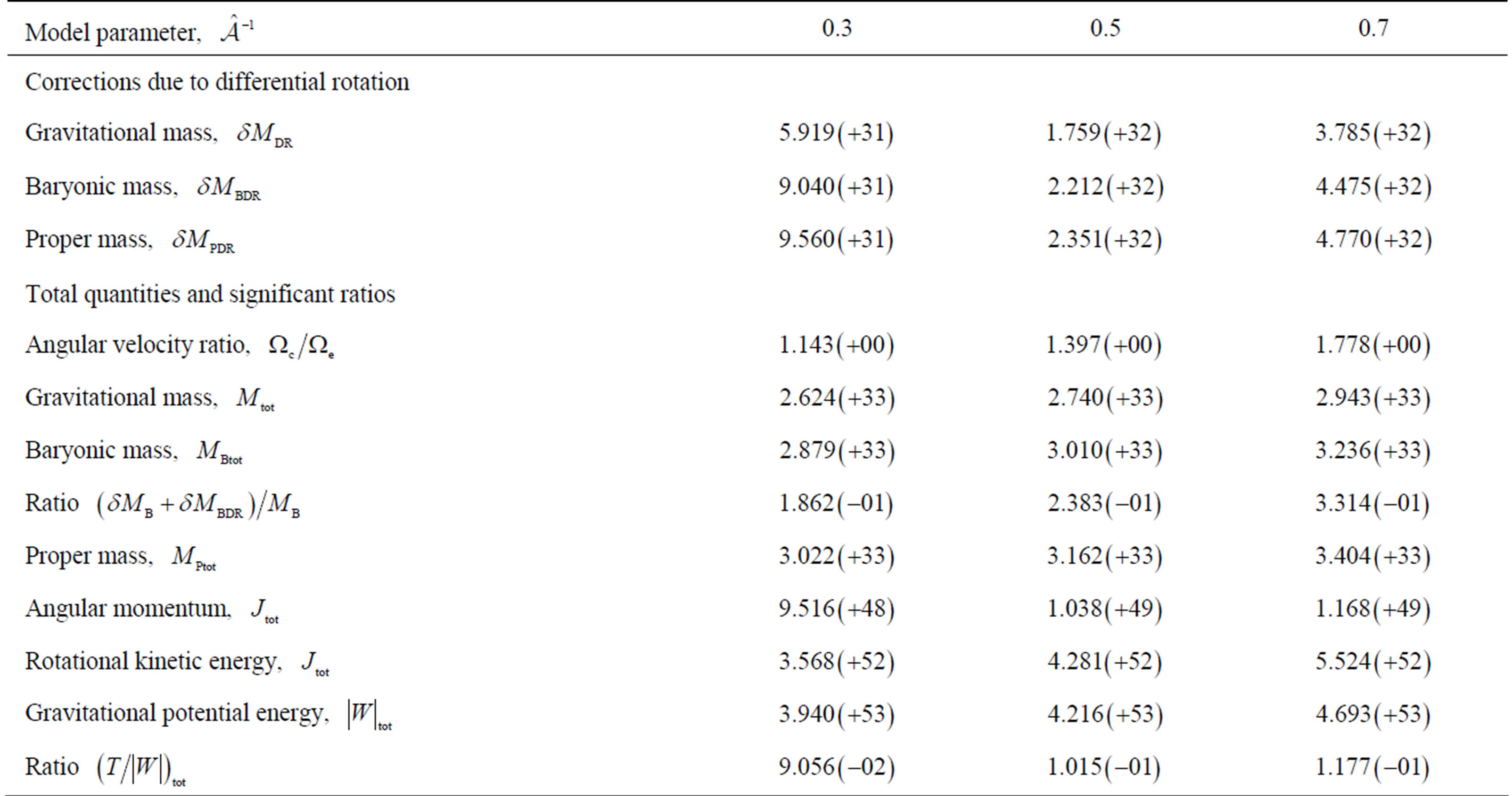
Table 5. Numerical results given in cgs for the EOS FPS; differential rotation for three values of the model parameter .
.

Table 6. Numerical results given in cgs for the EOS G; differential rotation for three values of the model parameter .
.
owing to differential rotation, we find that the ratio  takes its larger value for the EOS AU which is the most stiff among the EOSs examined. It is worth reminding here that, considering a group of EOSs, most stiff is the EOS yielding the larger pressure for a particular density, and most soft is the EOS yielding the smaller pressure for that density among the EOSs of the group. Note, in addition, that the EOSs AU, C, and FPS are compatible in their stiffness for the density
 , next is the EOS F and most soft in the group is the EOS G; for larger densities, AU clearly becomes the most stiff, C and FPS continue to be compatible, F is the next one, and G remains the most soft in the group. Sorting our EOSs this way, we find that the change in mass decreases with the stiffness of the EOSs.
The “equatorial differential rotation profiles” (EDRP)  are shown for our models in Figures 1, 3, 5, 7, and 9. Finally, Figures 2, 4, 6, 8, and 10 show the

Figure 2. Meridional cross section for the model obeying the EOS AU and for the value  (bold line; soft line: the unperturbed model).

Figure 4. Meridional cross section for the model obeying the EOS C and for the value  (bold line; soft line: the unperturbed model).

Figure 6. Meridional cross section for the model obeying the EOS F and for the value  (bold line; soft line: the unperturbed model).

Figure 8. Meridional cross section for the model obeying the EOS FPS and for the value  (bold line; soft line: the unperturbed model).

Figure 10. Meridional cross section for the model obeying the EOS G and for the value  (bold line; soft line: the unperturbed model).
“meridional cross sections” of our models when the parameter  takes its larger value studied here, i.e.
 .
.