American Journal of Computational Mathematics, 2011, 1, 219-225
doi:10.4236/ajcm.2011.14025 Published Online December 2011 (http://www.SciRP.org/journal/ajcm)
General Solution of Generalized (2 + 1)-Dimensional
Kadomtsev-Petviashvili (KP) Equation by Using the



GG-Expansion Method
Abdollah Borhanifar, Reza Abazari
Department of Mathematics, University of Mohaghegh Ardabili, Ardabil, Iran
Received May 5, 2011; revised May 28, 2011; accepted June 10, 20 11
Abstract
In this work, the

GG


-expansion method is proposed for constructing more general exact solutions of the
(2 + 1)-dimensional Kadomtsev-Petviashvili (KP) equation and its generalized forms. Our work is motivated
by the fact that the

GG


-expansion method provides not only more general forms of solutions but also
periodic and solitary waves. If we set the parameters in the obtained wider set of solutions as special values,
then some previously known solutions can be recovered. The method appears to be easier and faster by
means of a symbolic computation system.
Keywords:

GG


-Expansion Method, Generalized Kadomtsev-Petviashvili (KP) Equation, Hyperbolic
Function Solutions, Trigonometric Function Solutions
1. Introduction
Nonlinear evolution equations (NLEEs) have been the
subject of study in various branches of mathematical-
physical sciences such as physics, biology, chemistry, etc.
The analytical solutions of such equations are of funda-
mental importance since a lot of mathematical-physical
models are described by NLEEs. Among the possible
solutions to NLEEs, certain special form solutions may
depend only on a sing le combination of variables su ch as
traveling wave variables. In the literatu re, there is a wide
variety of approaches to nonlinear problems for con-
structing traveling wave solutions. Some of these ap-
proaches are the Jacobi elliptic function method [1], in-
verse scattering method [2], Hirotas bilinear method [3],
homogeneous balance method [4], homotopy perturba-
tion method [5], Weierstrass function method [6], sym-
metry method [7], Adomian decomposition method [8],
sine/cosine method [9], tanh/coth method [10], the
Exp-function method [11-16] and so on. But, most of the
methods may sometimes fail or can only lead to a kind of
special solution and the solution procedures become very
complex as the degree of nonlinearity increases.
Recently, the 
GG


troduced by Wang et al. [17], has become widely used to
-expansion method, firstly in-
search for various exact solutions of NLEEs [17-27]. The
value of the


GG

-expansion method is that one treats
nonlinear proby essentially linear methods. The
method is based on the explicit linearization of NLEEs
for traveling waves with a certain substitution which
leads to a second-order differential equation with con-
stant coefficients. Moreover, it transforms a nonlinear
equation to a simple algebraic computation.
The generalized (2 + 1)-dimensional Ka
blems
domtsov-Pe-
tviashivilli (gKP) equ ation given by

=0, >1
2
n
tx xxxyy
x
uuu uun

  
The objectives of this work are twofold. First, we de-
scribe the


GG

-expansion method. Second, we aim
to implemenresent method to obtain general exact
travelling wave solutions of governing equation.
t the p
2. Description of the



GG-Expansion
The objective of this section is to outline the use of the
Method


GG

-expansion method for solving certain nonlinear
ifferential equations (PDEs). Suppose we have a partial d
nonlinear PDE for


,, ,uxyt in the form

A. BORHANIFAR ET AL. 220
where is a polynomial in its argumen
cludes inear terms and the highest ord

,,,, ,=0,
xy
Puuu uu (1)
x txx
P
nonl
nsf
ts, which in-
er derivatives.
The traormation

,,, =uxyzt U

, =kx yt



,
reduces Equation (4) to the ordinary differential equation
(ODE)

2
,,, ,,=0,PU kUUkUkU 
 
 (2)
where =(),UU

and prime denotes derivat
respect tive with o

.
be expresse
We assume that the solution of Equation
(2) cand by a polynomial in

GG
 as fol-
lows:
 
0
=1
=,0
ni
in
i
UGG  

. (3)
where 0,

and ,
i

are constants to be determined
later, ()G

satisfies a second order linear ordinary dif-
ferential equation (LODE):




2
2
dd =0.
dd
GG
G



 (4)
where

and

are arbitrary constants. Using the ge-
neral solutions of Equation (4), we have


22
12
22
22
12
22
12
2
2
12
44
sinh cosh
22
4,4
22
44
cosh sinh
22
44
sin cos
22
4
24
cos sin
2
CC
CC
G
G
CC
CC
 
0,

 
 


 















 

























2
2,40,
2
4
2


























(5)
and it follows, from (3) and (4), that
 

 
1
=1
21 12
22
=1
,
=121(2) 211,
i
i
nii iii
i
i
GG
Ui iGGiGGiGGiGGiGG



 


 
 
 
 

(6)
and so on, here the prime denotes the derivative with
spective to
1
=
nii
i
UiGGGG 


 


re

.
To determine u explicitly, we take the following
four steps:
Step 1. Determin the integer n by substituting Equa-
tion (3) aloe ng with Equation (4) into Equation (2), and
ba nl
Equation (4) into Equ
tio
lancing the highest order noinear term(s) and the
highest order partial derivative.
Step 2. Substitute Equation (3) give the value of n
determined in Step 1, along witha-
fn (2) and collect all terms with the same order o

GG
 together, the left-hand side of Equation (2) is
converted into a polynomial in

GG
. Then set each
ent of this polynomial to zero to derive a set of
algebraic equations for 0
,,k
coeffici

 and i

.
Step 3. Solve the system of algebraic equations ob-
tained in Step 2, for 0
,,,,abc

 a ndi

by use of
Mobtained e
eries of fundamental solutions
aple.
Step 4. Use the results in abovsteps to de-
rive a s

u

of Equa-
tion (2) depending on


GG

, since the solutions of
Equation (4) have bn for us, then we can
ob
e
een well know
tain exact solutions of Equation (1).
3. Application
In this section, we will demonstrate th

GG

-dimension
-expan-
sion method on the generalized (2 + 1)al Ka-
ation given by domtsev-Petviashvili (KP) equ

=0,|
2
n
txxxx yy
x
uuu uun|>1,

   (7)
where ,

and

are constants. Using the wave vari-
able =,kx yt



 in (7) and integrating the result-
ing equation and neglecting the constant of i
we find ntegration,
22
140, 1,
21
n
kUkUn
n


 
kU 



our goal, we use the transformation



 (8)
To achieve

A. BORHANIFAR ET AL.221
 
,
n
UV
1

  that will carry (8) into the ODE
 

22
222234
111
2
nnkVknVnknVVnV


  
 



=0,
(9)
According to Step 1, we get2, hence
We then suppose that Equatioe fol-
lo
32mm
n (9) has th2.m
wing formal solutions:

2
21,0,VGG GG


 (10)
02
where 21
,,

 and 0,

are constants which
known to be determined later.
titutingon me order of
are un-
Subs Equati(10) into Equation (9) and col-
lecting all terms with the sa

GG




22 22
01
22
22 42 422
222
22 322 3
=,=
22 328
=,=
2
knnknn
nn
knn kk
nk
 



 

 


,
,
n
n
(11)
Substitute the above general case in (10), we get


to-
gether, the left-hand sides of Equation (9) are converted
into a polynomial in

GG
. Setting each coefficient of
each polynomial to zero, we derive a set of algebraic
equations for 01
,, ,k,,,



  and 2,

and
solving them by use of Maple, we get the following gen-
eral result:

22 2
22 3, knnGGG 
2
1, 2.
VG
n
nn









(12)
then use the transformation
 
1
=,
n
UV

when
,
240


 the hyperbolic function solutions of Equa-
tion (7), becomes:


2
2
4
cos


2
2
112
22
222
21
2
212
4
4sinh h
22
22 3
=2
44
2sinh cosh
22
4
4sinh cosh
2
nCC
knn
un
CC
CC

 



 

 
 

 


 





 

 


 




  


 





 






1
2
22
21
4
2,
2
44
2sinh cosh
22
n
CC


 















 


  

  
 


 




(13)
and when , the trigonometric function solutions of Equation (7), will be:
240
 


2
2
4 
2
2
112
22
222
21
2
212
4
4sin cos
22
22 3
2
44
2sin cos
22
44
4sin cos
2
nCC
knn
un
CC
CC

 



 

 
 






 
 

 

 




 



 




 











 








1
2
22
21
2,
2
44
2sin cos
22
n
CC


 





 
 

 






 
 

  
 








(14)
here w42 422
2
28
=,
2
kk n
kx yt
kn
 


  12
,,,CC

and

are arbitrary constants.
In particular, when then the general solutions
and
2=0,C

A. BORHANIFAR ET AL. 222
(13) and (14) reduces , res pectively,


12
42 22
2
28
2
kk n
kxyt
n
22 22 4
2
1
22 42 422
2
22 344
22 2
44 28
tanh ,
22 2 2
n
n
knn
nk
kk n
kx yt
kn
 
tanhu











 
   


 

 

 




  






  

 










(15)
 




1
2
t
n
2
22 22 42 4 22
2 2
1
22 42 422
2
22 344
28
tan
22 2
44
28
tan ,
22 22
n
n
knnkk n
ukxy
nk
kk n
kx yt
kn
 





  


 

 
 

 




  

 





   
















(16)
and when then we deduce from general solutions (13) and (14) that,
1=0,C


12
22 22 42 422
2 2
1
22 42 422
2
22 344
28
coth
22 2
44 28
coth ,
22 22
n
n
knnkk n
ukxy
nk
kk n
kx yt
kn
 
2
t
n





  





 
 

 




  


 




  















(17)






12
22 22 42 422
2 2
1
22 42 422
2
22 344
28
() cot
22 2
44 28
cot ,
22 2 2
n
n
knnkk n
ukxy
nk
kk n
kx yt
kn
 
2
t
n





  


 


 
  




 


 





  
















(18)
where ,, ,k

 and

are arbitrary constants.
For important case 3 =,
2
n



32 2=0
txxxxyy ,
x
uuuuu   
where
(19)
and

,

are constants, then according to re-
sults in (11), the general hyperbolic and trigonometric
function solution of (19) will be
the KP Equation (7) re-
duce to


23
222
1
35kC 





2
2
2
4
cosh 4
C
C









(20)
2
22
21
4
=,
11
18 sinh4
22
u
C



















23
22 22 2
12
22
222
2
212 12
35 44,
444
182 sincos
cos 222
kC C
u
CCC CC
 

 


2


 
 

 
 
  

 
 
 


 


 
(21)



A. BORHANIFAR ET AL.223
where and ,

42 42
41692
,
9
kk
kx yt
k
  


  
12
,,,,CC k


=0, then the ge
and μ are arbitrary constants. When
neral hyperbolic and trigonometric
function solution (20) and (21) reduce to
2
C


2
3
22
42 42
,
9
41 6
2
kk

 

 
(22)
2
35 4
4
18cos 29
k
u
kx yt
k
 





























2
3
22
42 42
2
2
35 4,
9
416
42
18cos 29
k
u
kk
kx yt
k












































(23)
and when then the general solution (20)-(21) reduce to
1=0,C


2
3
22
42 42






24
4kk 
2
35 4
=,
9
16
2
18sinh 29
k
u
kx yt
k
 
















 





















(24)



2
3
22
42 42
2
2
35 4.
9
416
42
18sin 29
k
u
kk
kx yt
k


 









































(25)
We would like to note that the obtained solutions with
an explicit linear function in

have been checked with
Maple by putting them back into the original Equations
(7).
4. Conclusions and Future Work
This study shows that the

GG

-expansion method is the equations considered, they might serve as seeding
quite efficient and practically well suited for use in find-
ing exact solutions for the ge
sional Kadomtsev-Petviashvili (gKP) equation. The reli-
ability of the method and the reduction in the size of
computational domain give this method a wider applica-
bility. Though the obtained solutions represent only a
small part of the large variety of possible solutions for
neralized (2 + 1)-dimen-

A. BORHANIFAR ET AL. 224
ical systems. Furthermore, our solutions are in m
general forms, and many known solutions to these equa-
he aid of Ma-
ple, we have assured the correctness of the obtained so-
k into
solutions for a class of localized structures existing in the
physore
tions are only special cases of them. With t
lutions by putting them bacthe original equation.
We hope that they will be useful for further studies in
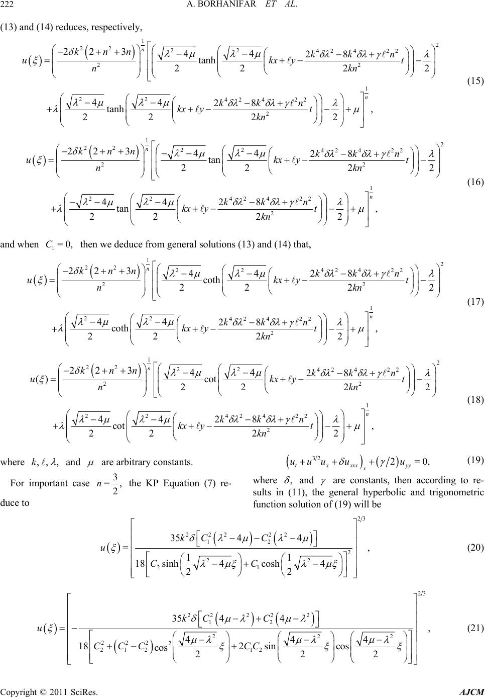
applied sciences. According to Case 5, present method
failed to obtain the general solution of gKP for =1,n

and =2,n therefore the authors hope to extend the

GG
-expansion method to solve these especial type
of gKP.
5. Acknowledgments
This work is partially supported by Grant-in-Aid from
the University of Mohaghegh Ardabili, Ardabil, Iran.
6. References
[1] G. T. Liu and T. Y. Fan, “New Applications of Devel-
oped Jacobi Elliptic Function Expansion Methods,” Phy-
sics Letters A, Vol. 345, No. 1-3, 2005, pp. 161-166.
doi:10.1016/j.physleta.2005.07.034
[2] . J. Ablowitz and H. Segur, “Solitons and Inverse Scat-
tering Transform,” SIAM, Philadelphia, 1981.
doi:1
M
0.1137/1.9781611970883
ethod in Soliton Theory,” Cam-
ambridge, 2004.
[3] R. Hirota, “The Direct M
bridge University Press, C
[4] M. L. Wang, “Exact Solutions for a Compound KdV-Burg-
er s Equation,” Physics Letters A, Vol. 213, No. 5-6, 1996,
pp. 279-287. doi:10.1016/0375-9601(96)00103-X
[5] J. H. He, “The
linear Oscillat Homotopy Perturbation Method for Non- ors with Discontinuities,” Applied Mathe-
matics and Computation, Vol. 151, No. 1, 2004, pp. 287-
292. doi:10.1016/S0096-3003(03)00341-2
[6] Z. Y. Yan, “An Improved Algebra Method and Its Ap-
plications in Nonlinear Wave Equations,” Chaos Solito
& Fractals, Vol. 21, No. 4, 2004, ppns . 1013-1021.
doi:10.1016/j.chaos.2003.12.042
[7] G. W. Bluman and S. Kumei, “Symmetries and
tial Equations,” Springer-Verlag Differen- , New York, 1989.
994.
ca
r Partial Dif-
ional Nizhnik-Novikov-
.064
[8] G. Adomian, “Solving Frontier Problems of Physics: The
Decomposition Method,” Kluwer, Boston, 1
[9] A. Borhanifar, H. Jafari and S. A. Karimi, “New Solitons and
Periodic Solutions for the Kadomtsev-Petviashvili Equa-
tion,” The Journal of Nonlinear Science and Applitions,
Vol. 1, No. 4, 2008, pp. 224-229.
[10] H. Jafari, A. Borhanifar and S. A. Karimi, “New Solitary
Wave Solutions for the Bad Boussinesq and Good Bous-
sinesq Equations,” Numerical Methods fo
ferential Equations, Vol. 25, No. 5, 2000, pp. 1231-1237.
[11] A. Borhanifar, M. M. Kabir and L. M. Vahdat, “New Pe-
riodic and Soliton Wave Solutions for the Generalized Zak-
harov System and (2 + 1)-Dimens
Veselov Sy stem,” Chaos Solitons & Fractals, Vol. 42, No.
3, 2009, pp. 1646-1654. doi:10.1016/j.chaos.2009.03
thod for
[12] A. Borhanifar and M. M. Kabir, “New Periodic and Soli-
ton Solutions by Application of Exp-Function Me
Nonlinear Evolution Equations,” Journal of Computa-
tional and Applied Mathematics, Vol. 229, No. 1, 2009,
pp. 158-167. doi:10.1016/j.cam.2008.10.052
[13] S. A. El Wakil, M. A. Abdou and A. Hendi, “New Peri-
odic Wave Solutions via Exp-Function Method,” Physics
Letters A, Vol. 372, No. 6, 2008, pp. 830-840.
doi:10.1016/j.physleta.2007.08.033
[14] A. Boz and A. Bekir, “Application of Exp-Function Me-
thod for (3 + 1)-Dimensional Nonlinear Evolution Equa-
tions,” Computers & Mathematics with Applications, Vol.
56, No. 5, 2000, pp. 1451-1456.
[15] H. Zhao and C. Bai, “New Doubly Periodic and Multiple
Soliton Solutions of the Generalized (3 + 1)-Dimensional
Kadomtsev-Petviashvilli Equation with Variable Coeffi-
cients,” Chaos Solitons & Fractals, Vol. 30, No. 1, 2006,
pp. 217-226. doi:10.1016/j.chaos.2005.08.148
[16] M. A. Abdou, “Further Improved F-Expansion and New
Exact Solutions for Nonlinear Evolution Equations,” Non-
linear Dynamics, Vol. 52, No. 3, 2008, pp. 277-288.
doi:10.1007/s11071-007-9277-3
[17] M. Wang, X. Li and J. Zhang, “The (G'/G)-E
Method and Traveling Wave Solutioxpansion ns of Nonlinear Evo-
lution Equations in Mathematical Physics,” Physics Let-
ters A, Vol. 372, No. 4, 2008, pp. 417-423.
doi:10.1016/j.physleta.2007.07.051
[18] J. Zhang, X. Wei and Y. J. Lu, “A Generalized (G'/G)-
Expansion Method and Its Applications,” Physics Letters
A, Vol. 372, No. , 2008, pp. 36-53.
doi:10.1016/j.physleta.2008.01.057
[19] A. Bekir, “Application of the (G'/G)-Expansion Method
for Nonlinear Evolution Equations,” Physics Letters A,
ons
Vol. 372, No. 19, 2008, pp. 3400-3406.
[20] A. Bekir and A. C. Cevikel, “New Exact Travelling Wave
Solutions of Nonlinear Physical Models,” Chaos Solit
& Fractals, Vol. 41, No. 4, 2008, pp. 1733-1739.
[21] E. M. E. Zayed and K. A. Gepreel, “Some Applications
of the (G'/G)-Expansion Met hod to Non -Linear Pa rtial Dif-
ferential Equations,” Applied Mathematics and Computa-
tion, Vol. 212, No. 1, 2009, pp. 1-13.
doi:10.1016/j.amc.2009.02.009
[22] D. D. Ganji and M. Abdollahzadeh, “Exact Traveling So-
lutions of Some Nonlinear Evolution Equation by (G'/G)-
Expansion Method,” Journal of Ma
Vol. 50, No. 1, 2009, Article ID: 013thematical Physics, 519.
doi:10.1063/1.3052847
[23] M. Wang, J. Zhang and X. Li, “Application of the (G'/G)-
Expansion to Travelling Wave Solutions of the Broerkaup
and the Approximate Long Water Wave Equations,” Ap-
plied Mathematics and Computation, Vol. 206, No. 1, 2008,
pp. 321-326. doi:10.1016/j.amc.2008.08.045
[24] L.-X. Li and M.-L.Wand, “The (G'/G)-Expansion Method
and Travelling Wave Solutions for a Higher-Order Non-
linear Schrdinger Equation,” Applied Mathematics and
Computation, Vol. 208, No. 2, 2009, pp. 440-445.
doi:10.1016/j.amc.2008.12.005

A. BORHANIFAR ET AL. 225
reel, “The (G'/G)-Expan-[25] E. M. E. Zayed and K. A. Gep
sion Method for Finding Traveling Wave Solutions of
Nonlinear Partial Differential Equations in Mathematical
Physics,” Journal of Mathematical Physics, Vol. 50, No.
1, 2008, Article ID: 013502. doi:10.1063/1.3033750
[26] I. Aslan and T. Ozis, “Analytic Study on Two Nonlinear
, Vol. 209,
No. 2
Evolution Equations by Using the (G'/G)-Expansion Me-
thod,” Applied Mathematics and Computation
, 2009, pp. 425-429. doi:10.1016/j.amc.2008.12.064
[27] I. Aslan and T. Ozis, “On the Validity and Reliability of
the (G'/G)-Expansion Method by Using Higher-Order Non-
linear Equations,” Applied Mathematics and Computation,
Vol. 211, No. 2, 2009, pp. 531-536.
doi:10.1016/j.amc.2009.01.075