ABSTRACT

In this work, we analyzed the impact of interventions on populations which exhibit unimodal dynamics. The six landmarks that characterize the “shape” of the unimodal reproduction curve of the difference equation, , are defined and used in order to examine and determine the behavior of dynamics of populations. By using the Li-Yorke criterion for determination of chaos we propose a qualitative intervention rule that can be applied without any explicit population equation. This proposed strategy for intervention brings out many interesting behaviors in population dynamics. A qualitative decision rule can be applied with a straight edge without any population equation and therefore offers a robust strategy for the management of populations.

1. Introduction

When we intervene in ecosystems in order to reduce populations of pests and parasites or enhance populations of fish or pollinators, we confront systems that have their own dynamics. Our interventions are usually aimed at changing the mean population size in a way guided by plausible common sense. If we want to reduce a population, kill them. If we want to increase a population, release fry or fledglings. There are examples of trying to control populations such as dangue by spraying insect pesticide against the mosquito vectors [1,2]. The use of pesticides is a common practice in agriculture, and their roles have been descried in [3].

However, our interventions affect more than the mean values of target species. They percolate through a network of interacting species, are amplified along some pathways, buffered along others, and may even be reversed. They also alter the dynamics of populations, their equilibrium values, their age distribution, their local and global stability, periodic oscillations and even may induce or eliminate chaotic dynamics. For example, chaotic dynamics can appear from a time-delayed inhibitory effect of plant litter on subsequent growth when we increase the productivity of the plant [4]. Another example is the effect of global warming on the population dynamics of the Lyme disease vector [5].

It was also shown theoretically and experimentally that small perturbations can affect the dynamics of an insect population at its three developmental stages [6].

In this paper we examine the impact of interventions on populations which exhibit unimodal dynamics, using six landmarks. That is, we consider cases in which the dynamics of a population are described by an equation of the form,

(1)

where X_n is the population size at time n, the function is non-negative, , increases with x up to some peak value and then declines. There are many possible mathematical forms for. But here we do not specify the equation. The unimodal shape by itself provides guidelines for analysis, and the study fits into our strategy of qualitative mathematical biology that asks the question, “what can we get away without knowing and still understand the system enough to make reasonable decisions about interventions.”

2. The Web Map and the Trajectory

The unimodal shape is often a reasonable assumption for a reproduction curve. For instance, for modeling the dynamics of the growth of grass in a savanna, the shape of reflects the fact that the quantity of grass present affects growth in opposing ways: by way of reproduction, the more grass now the more grass later, but through litter accumulation on the ground, old grass inhibits new growth. Therefore, the curve would start at zero, rise to some peak level, and taper off asymptotically toward zero when litter completely covers the ground and suppresses growth [7].

Successive values of x can be traced by the web map as shown in Figure 1(a). From any initial value x₀ on the x_n axis, we draw a vertical line to the curve, then a horizontal line to the bisector x_n+1 = x_n and repeat the process: vertical to the curve, horizontal to the bisector. As in Figure 1(b), we can connect the curve to the time course. You may start from any initial value x₀. Where the bisector intersects with the curve we have the positive equilibrium of the Equation (1). This equation exhibits negative feedback: if x_n is above equilibrium then x_n+1 < x_n while if x_n is below equilibrium then x_n+1 > x_n. The trajectory of x (the solution to Equation (1)) may approach the equilibrium or oscillate permanently. It may be below equilibrium for several consecutive steps, but can only be above equilibrium for a single step.

3. The Six Landmarks to Understand the “Shape” of the Curve

We take a simple qualitative approach for understanding the dynamics from the shape of the curve [8]. In Figure 2, the equilibrium value x^* is one of six crucial landmarks that show the dynamics. The others are: the peak P, at which reaches its maximum value. The maximum value, , and the minimum value, , together bound the region of permanence. If x_n is in the region of permanence then all subsequent values are in that region, while if x_n is a positive number outside the region of permanence then the trajectory will return to this region.

The other landmarks are pre-images. In a previous study the structure of pre-image sets were mathematically analyzed in the context of a two species competetion model based on a system of two difference equations [9]. In our work the pre-images are used as indicators along with others for qualitative studies.

The first negative pre-image y₋₁ is the value of x_n from which x_n+1 = x^*. That is,. The second negative pre-image is that value for x for which and so on:. In order to create graphically and, you start from the equilibrium x^*, then a horizontal line back to the curve, next a vertical line to the bisector x_n = x_n+1, then go horizontally back to the curve, and you can find. If x_n lies between and, then x_n+1 lies between and. That is, a trajectory crosses one pre-image in each iteration. From the figure we see that there are no positive pre-images. Therefore, if x_n is above

equilibrium, then x_n+1 is below the equilibrium. The 6 landmarks are shown in Figure 2, as highlighted in red.

The local stability of the dynamics around the equilibrium depends on the slope of the curve at equilibrium. If at x^* lies between −1 and 1, then the equilibrium is locally stable. If instead the equilibrium is unstable and the trajectory is periodic, then the period is stable if the product of the slopes around the cycle is between −1 and 1. Notice that it is possible to have a curve that gives a locally stable equilibrium and yet is chaotic because the chaotic properties depend on the relations among the landmarks.

4. The Li-Yorke Criterion for Determination of Chaos

Li and Yorke [10] showed that if we can find a sequence in the solution of Equation (1) such that_, then the following are true:

1) The Equation (1) has solutions of every integral period;

2) There are non-periodic solutions;

3) There is extreme sensitivity to initial conditions.

These three properties of a non-delay difference equation together define chaos, an unfortunate term since it implies total disorder, whereas chaotic dynamics do in deed have regularities.

Applying the Li and Yorke criterion, we find that if lies in the permanent region, then Equation (1) is chaotic. This is equivalent to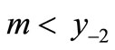. If is in the region of permanence then there will be sequences below equilibrium from of length at least k before crossing over x^*. Note: the negative semi-cycle (the number of consecutive iterations below equilibrium) may be limited to less than some k whereas there are solutions of all periods. This means that periodic orbit may cross equilibrium several times before returning to a previous value. The semi-cycle is more readily determined than the period since we cannot tell when a value is exactly at some pervious value but we can see the inter-peak (the sum of the negative and positive semi-cycles).

Note that whereas local stability around equilibrium depends on the slope at the equilibrium, the determination of chaos depends on the “shape” of the function as determined by the 6 landmarks.

5. Interventions

A policy is some rule of intervention that changes for some values of x. A common rule in economic entomology is the economic threshold: intervene when the pest population exceeds some threshold value determined by the amount of damage the pest causes, the cost of corresponding crop losses, and the cost of the intervention. Threshold concepts provide guidelines to reduce the total amount of pesticides applied, while maintaining or improving farm profitability. More details on economic threshold can be found in [11].

Suppose now that the threshold for intervention is located above the equilibrium value (Threshold 1 in Figure 3(a)). It lowers the unimodal curve on the right of Threshold 1 as described in Figure 3(a). This has no effect on the equilibrium x^*, the peak P, the maximum M or the pre-images, but is lowered. If the equation was previously stable, m might now be below y₋₂ and the dynamics may become chaotic as in Figure 3(c).

If the previous dynamics was locally stable, the solution may behave chaotically until it falls within the interval around x^* where the slope is flatter than −1, and then x oscillates into equilibrium.

It is not obvious whether chaos is desirable or not. If damage to the crop is proportional to the pest population, since oscillation reduces the mean of x, chaos might be beneficial. But if the crop can tolerate a certain level of damage but suffers losses when the pest population peaks, then oscillations may be harmful. Therefore it is important to propose an intervention strategy that pertains to our goal.

A lower threshold for intervention (for example, Threshold 2 in Figure 3(a)) can reduce the equilibrium value as well as provoke chaos. Then x^* and the pre-images are reduced and it is not obvious whether the pre-image is now above or below m.

If intervention occurs only when the population is expanding most rapidly, the peak P will be lowered as described in Figure 4(a). This reduced M, which in turn increases m. Therefore this intervention may eliminate chaos if m is now above the pre-image. The trajectory became stable as the intervention changed the region of permanence.

Now suppose that our interest is in preserving a species. Sometimes a small population is not able to grow because members of the population cannot find a mate. For instance, there are two trees in a neighborhood, but they are too far to exchange the pollens; a population is endangered if it gets too small. Therefore a rule for intervention would be that when x is below some threshold we add some number of the plants. Another example of this kind of intervention is the addition of salmon fish when the population is low in a salmon farm [12].

In our example described in Figure 5(a), there exist two equilibrium points on the original curve (the blue curve) before intervention; an unstable equilibrium to the left of the peak and the other equilibrium to the right of the peak. The variable either can go to the left or to the right, but can’t stay at the unstable equilibrium. By the Li-Yorke criterion, the second pre-image of the original curve placed above the minimum essentially implies chaos. Also notice that the unstable equilibrium (0.114) was placed slightly above the minimum (0.1085) on the original curve. Thus, as in Figure 5(b), the population behaves chaotically until it gets caught up below the unstable equilibrium, and then dies out to zero.

However if our intervention bulges to the left for small values as described in Figure 5(a), then the only effect on the landmarks is to move the pre-images to the left if they are already below the threshold. Therefore it may place some of them outside the region of permanence. This reduces the number of steps in the semi-cycle and if is moved to the left of m then there will be no chaos.

Since we don’t specify the exact functional shape, we don’t know exactly whether this intervention will place both of the pre-images below the minimum. In this example of in-

tervention, the previously unstable equilibrium was removed, but the minimum is now placed in between y₋₂ and, so the determination of chaos is not obvious in this case. As in Figure 5(c), it turns out that the population still exhibits a chaotic behavior. However, our intervention strategies using the six land marks suggest some directions for the management of population.

If what we want is a stable trajectory, then we can intervene again when the population is expanding most rapidly by removing some animals when they are near the peak as in Figure 6(a). The peak area of the curve is again cut off. This decreases the maximum, which in turn increases the minimum, placing y₋₁ below the minimum, and it removes chaos as in Figure 6(c).

Suppose now the curve represents the pests in agriculture, and we want to protect the harvest. We need to know what the nature of the harm the insect causes is. If an insect eats proportional to the population, then the amount of damage the insect causes is proportional to the mean population of insects. Suppose you have a chaotic population. The population oscillates in a chaotic way, but its average is going to be less than or equal to the equilibrium as oscillation reduces the mean of x. In this situation chaos can be beneficial to the harvest.

It is also possible that the damage the insect causes mostly occurs at peaks. For example, plants can grow when they lose some leaves, but if they lose lots of leaves, then they may not be able to survive; sometimes the peak causes the plants the troubles and sometimes the average does. That is something we have to decide from the nature of the circumstances. If the peaks cause the plants troubles, and a chaotically behaving insect population gets really big, then you can intervene to add number of insects when the insect population is above a certain threshold. Although this intervention is different from what conventional wisdom would indicate, we raise the minimum by this intervention, so the minimum now becomes greater than both y₋₁ and y₋₂. This change in its landmarks suppresses chaos, reducing the damages that occur at peaks, while it does not affect the equilibrium.

Consider now that applies to the pest population in a crop of beans. Consider the intervention strategy of increasing a loan to encourage farmers to plant several crops of beans per year with less time between crops, as described in the equation, , where r is greater than 1. This intervention steepens all slopes and makes periodic and chaotic solutions more likely. In this way, our interventions generally affect the stability of solutions [8].

6. Conclusions

This kind of qualitative analysis and intervention strategies is more robust than the more precise models that give explicit equation for because it makes fewer restrictive and usually unrealistic assumptions about the shape of that function. Our intervention strategies depend on what the natural content of the population we are working with is, and the objects that we try to manage. Then we can think of how to intervene to get those results by this kind of qualitative analysis.

The dynamics of the difference equation without delays (1) can be grasped quickly and intuitively from ex-

amining the “shape” of the curve. In order to do so, we have to look at in terms of its landmarks: the equilibrium value x^*, the peak, the boundaries of the permanent region M and m, and the pre-image set. As a consequence, a qualitative decision rule can be applied with a straight edge without any population equation and therefore offers a robust strategy for the management of populations.

In the case of difference equations without delay, we have demonstrable results. For equations with delay, or for differential equations, there are fewer analytic results, but the qualitative conclusion above can be used as working hypotheses that can guide explorations by numerical methods and analysis for other cases [8].

REFERENCES

- T. Awerbuch, R. Levins and M. Predescu, “Co-Dynamics of Consciousness and Populations of the Dengue Vector in a Spraying Interventions System Modeled by Difference Equations,” Far East Journal of Applied Mathematics, Vol. 37, No. 2, 2009, pp. 215-228.
- M. C. Akogbeto, R. Djouaka and H. Noukpo, “Use of Agricultural Insecticides in Benin,” Bulletin de la Société de Pathologie Exotique, Vol. 98, No. 5, 2005, pp. 400- 405.
- Food and Agriculture Organization of the United Nations, “International Code of Conduct on the Distribution and Use of Pesticides,” 2002. http://www.fao.org/waicent/faoinfo/agricult/agp/agpp/pesticid/code/download/code.pdf
- D. Tilman and D. Wedin, “Oscillations and Chaos in the Dynamics of a Perennial Grass,” Nature, Vol. 353, 1991, pp. 653-655. http://dx.doi.org/10.1038/353653a0
- T. Awerbuch, A. Kiszewski and R. Levins, “Surprise, Nonlinearity and Complex Behavior,” In: Martens and Mcmichael, Eds., Health Impacts of Global Environmental Change: Concepts and Methods, 2002, pp. 96-102.
- R. A. Desharnais, B. Dennis, J. M. Cushing, S. M. Henson and R. F. Costantino, “Chaos and Population Control of Insect Outbreaks,” Ecology Letters, Vol. 4, No. 3, 2001, pp. 229-235. http://dx.doi.org/10.1046/j.1461-0248.2001.00223.x
- E. A. Grove, G. Ladas, R. Levins and C. Puccia, “Oscillation and Stability in Models of a Perennial Grass,” Proceedings of. Dynamic Systems & Applications, Vol. 1, 1994, pp. 87-91.
- R. Levins, “The Butterfly ex Machine,” In: R. S. Singh and C. B. Krimbas, Eds., Evolutionary Genetics: From Molecules to Morphology, Cambridge University Press, Cambridge, 2000, pp. 529-543.
- Y. Kang, “Pre-Images of Invariant Sets of a Discrete- Time Two-Species Competition Model,” Journal of Difference Equations and Applications, Vol. 18, No. 10, 2012, pp. 1709-1733.
- T. Y. Li and J. Yorke, “Period Three Implies Chaos,” The American Mathematical Monthly, Vol. 82, No. 10, 1975, pp. 985-992. http://dx.doi.org/10.2307/2318254
- A. Weersink, W. Deen and S. Weaver, “Defining and Measuring Economic Threshold Levels,” Canadian Journal of Agricultural Economics, Vol. 39, No. 4, 1991, pp. 619- 625. http://dx.doi.org/10.1111/j.1744-7976.1991.tb03613.x
- M. Krkosek, M. A. Lewis, A. Morton, L. N. Frazer and J. Volpe, “Epizootic of Wild Fish Induced by Farm Fish,” Proceedings of the National Academy of Sciences of the United States of America, Vol. 103, No. 42, 2006, pp. 15506-15510. http://dx.doi.org/10.1073/pnas.0603525103