American Journal of Computational Mathematics
Vol. 3 No. 2 (2013) , Article ID: 33548 , 11 pages DOI:10.4236/ajcm.2013.32023
Computational Studies of Bacterial Colony Model
Department of Mathematics, Faculty of Nuclear Sciences and Physical Engineering, Czech Technical University in Prague, Prague, Czech Republic
Email: partlond@fjfi.cvut.cz
Copyright © 2013 Ondřej Pártl. This is an open access article distributed under the Creative Commons Attribution License, which permits unrestricted use, distribution, and reproduction in any medium, provided the original work is properly cited.
Received January 17, 2013; revised February 24, 2013; accepted April 1, 2013
Keywords: Bacterial Colony Model; Reaction-Diffusion Equations; Method of Lines; Galerkin Finite Element Method
ABSTRACT
Microbiological experiments show that the colonies of the bacterium bacillus subtilis placed on a dish filled with an agar medium and nutrient form varied spatial patterns while the individual cells grow, reproduce and migrate on the dish in clumps. In this paper, we discuss a system of reaction-diffusion equations that can be used with a view to modelling this phenomenon and we solve it numerically by means of the method of lines. For the spatial discretization, we use the finite difference method and Galerkin finite element method. We present how the spatial patterns obtained depend on the spatial discretization employed and we measure the experimental order of convergence of the numerical schemes used. Further, we present the numerical results obtained by solving the model in a cubic domain.
1. Introduction
According to microbiological experiments, the colonies of the bacterium bacillus subtilis placed on a dish filled with an agar medium and nutrient form varied—and surprisingly regular—patterns while the individual cells grow, reproduce and migrate on the dish in clumps (see, e.g., [1,2]). As bacterium is an extremely primitive organism, the question arises whether the motion of the cells is governed by some simple underlying principles that can be described by mathematically.
The general approach to the pattern formation in biology is based on continuous and discrete dynamical models or neural models as described in [3]. In this case, the simple character of the motion of the bacteria resembles the Brownian motion and indicates the analogy with the diffusion limited aggregation (see [4]). Detailed analysis of the results of the experiments coupled the diffusion effects with the reactive behaviour of the species and led to the derivation of the model based on the reaction-diffusion system (see [5,6]) which was studied in [2,7]. In this article, we discuss it with respect to the accuracy and reliability of the numerical solution.
The model is based on the assumption that the cells can be divided into two classes: the active and the inactive. The active cells, with concentration  at the point x and time t, grow, move, feed on the nutrient and reproduce; whereas the inactive ones, with concentration
 , do not do anything. Finally, let
  be the concentration of the nutrient.
Then the time and space evolution of the concentrations within a bounded spatial domain , with
  or
or , is governed by the system
 (1)
(1)
 (2)
(2)
 (3)
(3)
for  and
and , where d represents a diffusion coefficient, and the function
  is of the form

with positive constants . The system (1)-(3) is subject to the initial conditions
 (4)
(4)
for  where
where  are
are  functions (
 represents the closure of
 ), and
  is a positive constant; and the boundary conditions

where  denotes the boundary of
 , and
, and  stands for the derivative of
  in the direction of the unit outward normal.
This problem can be written in the following weak formulation:
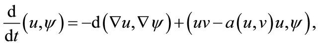 (5)
(5)
 (6)
(6)
for all  from the Sobolev space
  in the sense of distributions on a time interval
 , where
  stands for the inner product
 , where
 ;
;
 (7)
(7)
for all  in the sense of distributions on
 ; and
; and
 (8)
(8)
where .
.
The existence and uniqueness of the weak solution are proved in [8]. The authors also proved that

for a positive constant , and that there is a function
  (a final colony pattern) such that

Figure 1 shows the observed types of the spatial pat-

Figure 1. Types of the spatial patterns in  produced by the model studied. The patterns D-H correspond to the results of microbiological experiments. The results A-C have not been found in literature.
terns in  (the darker points correspond to the higher concentration of the cells) that have been found by the author by solving system (1)-(3).
2. Numerical Schemes
The model under consideration was solved numerically by means of the method of lines; for the spatial discretization, the finite difference method and Galerkin finite element method (the latter only in the case ) were used. For the sake of simplicity, we use only square and cubic domains
 , specifically

and
 .
.
2.1. Finite Difference Method
In the two-dimensional case, the domain  is covered by a regular orthogonal mesh of
  nodes
nodes with the step
 . Let us denote
 (
( and
and  are defined similarly). The spatial derivatives in (1) and (2) are approximated by the second order central difference, and the derivatives in the boundary conditions are approximated by the first order backward difference. Therefore, we obtain the following system of ODE’s:
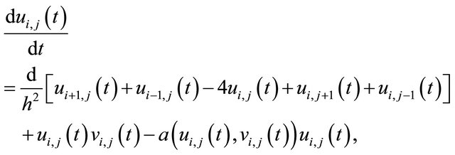


where in the first two equations, ; and in the third equation,
  Further, on the boundary we get

for ;
;

This system is supplemented with the initial conditions

where .
.
In the case of the cubic domain , the spatial discretization is derived analogically. These two schemes will be called MOL.
2.2. Galerkin Finite Element Method
In this method, both the linear (triangular) and the bilinear (square) Lagrange elements (see [9]) are used. The basis  of the finite dimensional subspace
 consists of the functions which are linear on each triangle (in the first case) or bilinear on each square (in the second case) and take the value 1 at one node of the spatial mesh and vanish at the other nodes. In the first case, two types of triangulations are used; they are depicted in Figure 2. In the case of the square finite elements, the same spatial mesh as in the method of lines is utilized. Further, the integrand in
  in (5) is approximated by its interpolant (see [9]). Finally, the numerical scheme is simplified employing the method of lumped masses (see [10,11]).
Hence, writing
 (9)
(9)
where Nh is the number of the nodes of the spatial mesh, Equations (5)-(7) are transformed as follows:
 (10)
(10)
 (11)
(11)
 (12)
(12)
for , where
  stands for the interpolant.
This system is supplemented with the initial conditions

where .
.
The schemes corresponding to the cases depicted in Figure 2 will be denoted FEMHS, FEMRHS and FEMSS, respectively.
The convergence of the numerical schemes derived can be proved as in [12-14]. The systems of ODE’s derived were solved by means of the Runge-Kutta-Merson method (see [12,15]) with the adaptive time step control.
3. Quantitative Studies
In the two-dimensional case, the experimental order of convergence (EOC), see [16], was measured; only the error of the functions u and v was considered. As the model studied does not possess an analytical solution, Equations (1) and (2) were transformed into the form
 (13)
(13)
where the additional terms  and
and  assure that the system possesses the solution

where  are positive constants.
Therefore, it turns out that


Figure 2. Meshes used for the Galerkin FEM.
and  (from the boundary conditions).
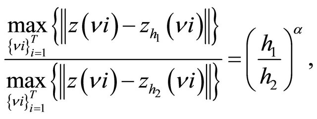
The modified system was solved analogically as the original one (the functions f and g were approximated in the same way as the functions u and v in (9)). The EOC coefficient  is defined by
 (14)
(14)
where ,
,  represents the numerical solution corresponding to the parameter
  which denotes the constant distance between two nodes on the bottom side (according to Figure 2) of the spatial mesh used (there are N nodes on this side), and
  denotes a suitable norm. The following form of Equation (14) was used:
 (15)
(15)
where  stands for a final time, and
  is a time step between the compared time levels of the solution. Two norms
  were used:


with

where  denote the nodal values of the projections of
  and
and  onto a regular orthogonal mesh with a spatial step
 .
.
The parameters were chosen as follows: L = 1,  ,
,
 ,
,  ,
,  ,
,  and
and . Further,
  (for the schemes FEMRHS, FEMHS and FEMSS) or
  (for the scheme MOL),
 ; and the mesh for the evaluation of the error had
  nodes
nodes .
.
The results are summarized in Tables 1-4. The EOC coefficients in the i-th row are computed from the data in the i-th and  -th row. The schemes FEMRHS, FEMHS and FEMSS exhibit the second order of convergence in h, and MOL exhibits the first order. Further,

Table 1. Results of the EOC measurement for the scheme MOL.

Table 2. Results of the EOC measurement for the scheme FEMSS.

Table 3. Results of the EOC measurement for the scheme FEMHS.

Table 4. Results of the EOC measurement for the scheme FEMRHS.
FEMSS appears to be the most accurate of all.
4. Computational Studies of Pattern Formation
This section provides the comparison of final spatial patterns obtained by the four schemes under consideration in a square domain. All the results were computed for
 and
and  (similarly as in the articles [2] or [7]); and the initial conditions were of the form

The function  was chosen constant. Therefore, the pattern types vary depending on the values of the parameters
  and
and .
.
The results presented (Figures 3-11) have the form of coloured pictures with a final shape of the function w, computed by one of the schemes, in shades of grey; each of the coloured lines in these pictures traces the spatial shape of the function w computed by one of the schemes for one value of N. Further, in Tables 5-7 there are differences between these shapes expressed by means of the  - and
- and  -norm (plus one another table for the combination
 ,
, ). The value of the
  - norm is divided by the area of
 . The time evolution of the patterns is shown in [17].
Note that, in general, it cannot be stated that one scheme is more or less accurate than the other schemes because, typically, each of them produces another shape. In author’s opinion, the most significant difference between the schemes consists in the symmetry of the results obtained by the scheme FEMHS.

Figure 3. Comparison of the schemes for v0 = 0.1, d = 0.05 and N = 1601.

Figure 4. Comparison of the schemes for v0 = 0.071, d = 0.12 and N = 1601.

Figure 5. Comparison of the schemes for v0 = 0.087, d = 0.05 and N = 1601.

Figure 6. Comparison of the schemes for v0 = 0.09, d = 0.1 and N = 1601.

Figure 7. Comparison of the schemes for v0 = 0.055, d = 0.1 and N = 1601.
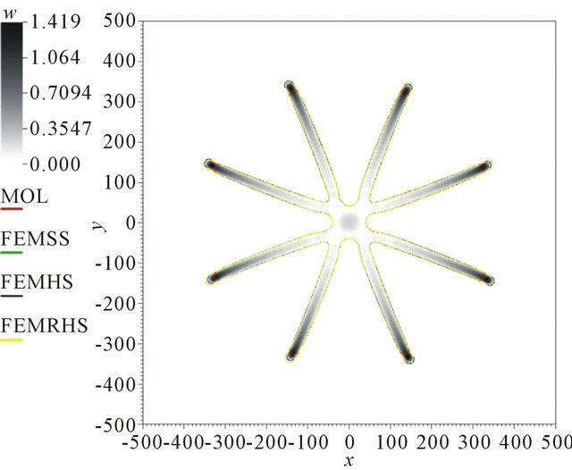
Figure 8. Comparison of the schemes for v0 = 0.06, d = 0.1 and N = 1601.

Figure 9. Comparison of the schemes for v0 = 0.065, d = 0.1 and N = 1601.

Figure 10. Comparison of the patterns computed by the scheme MOL for v0 = 0.065, d = 0.1 and different values of N.

Figure 11. Comparison of the patterns computed by the scheme FEMHS for v0 = 0.1, d = 0.05 and different values of N.

Table 5. Comparison of the final shapes of the function w. The shapes compared are depicted in Figures 3-6. In the case v0 = 0.25, d = 0.25, the results are too similar to be compared graphically.

Table 6. Comparison of the final shapes of the function w. The shapes compared are depicted in Figures 7-9.

Table 7. Comparison of the final shapes of the function w computed by one scheme with different values of N. The shapes compared are depicted in Figures 10 and 11.
5. Three-Dimensional Pattern Formation
This section provides examples of the spatial patterns that arise if we consider the cubic domain with  or
or . Similar types of the initial conditions and values of the parameters as in the two-dimensional case were used, i.e.,
  ,
,  and
and ;
;

( denotes the third spatial coordinate). The values of
  and
and  represented variable parameters of the model.
The results are presented in Figures 12-25. They have the form of coloured isolines of the functions u, v or . The time evolution is shown only for one combination of parameters; in the other cases, the solution evolves analogically.
6. Conclusions
It follows from the numerical results that the shape of the numerical solution strongly depends on the spatial discretization employed. The pattern type, nevertheless, seems to be stable, if the spatial mesh is not too coarse. In author’s opinion, therefore, the numerical methods under consideration can be used for the investigation of the pattern growth described by the system of the reaction-diffusion equations discussed.
As for the measurement of the experimental order of convergence, it is remarkable that the method of lumped masses does not seem to decrease it. Finally, the threedimensional model exhibits very complex behaviour as well.
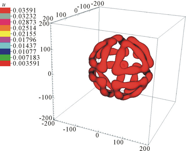
Figure 12. Isolines of u for L = 200, N = 201, v0 = 0.06 and d = 0.1 at t = 2500.

Figure 13. Isolines of u for L = 200, N = 201, v0 = 0.06 and d = 0.1 at t = 3500.
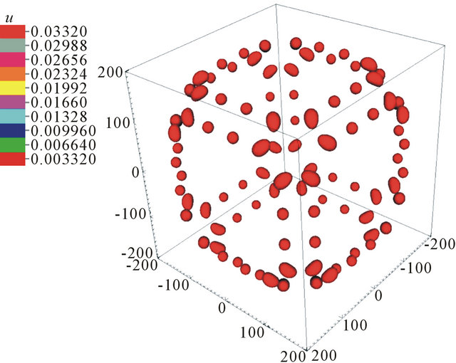
Figure 14. Isolines of u for L = 200, N = 201, v0 = 0.06 and d = 0.1 at t = 6500.

Figure 15. Isolines of v for L = 200, N = 201, v0 = 0.06 and d = 0.1 at t = 6500.

Figure 16. Isolines of u for L = 200, N = 201, v0 = 0.06 and d = 0.1 at t = 8000.

Figure 17. Isolines of u + w for L = 200, N = 201, v0 = 0.06 and d = 0.1 at t = 8000.

Figure 18. Isolines of u + w for L = 200, N = 201, v0 = 0.055, d = 0.1 and t = 13,000.

Figure 19. Isolines of u + w for L = 200, N = 201, v0 = 0.065, d = 0.1 and t = 9000.

Figure 20. Isolines of u + w for L = 200, N = 201, v0 = 0.07, d = 0.1 and t = 6000.

Figure 21. Isolines of u + w for L = 300, N = 301, v0 = 0.1, d = 0.05 and t = 6000.

Figure 22. Isolines of u + w for L = 300, N = 301, v0 = 0.071, d = 0.12 and t = 6000.

Figure 23. Isolines of u + w for L = 300, N = 301, v0 = 0.087, d = 0.05 and t = 12,000.

Figure 24. Isolines of u + w for L = 300, N = 301, v0 = 0.09, d = 0.1 and t = 6000.

Figure 25. Isolines of u + w for L = 300, N = 301, v0 = 0.25, d = 0.25 and t = 800.
7. Acknowledgements
Partial support of the projects “Applied Mathematics in Physics and Technical Sciences” number MSM684077 0010 of the Ministry of Education, Youth and Sports of the Czech Republic and “Advanced Supercomputing Methods for Implementation of Mathematical Models” number SGS11/161/OHK4/3T/14 is acknowledged.
REFERENCES
- J. Wakita, H. Shimada, H. Itoh, T. Matsuyama and M. Matsushita, “Periodic Colony Formation by Bacterial Species Bacillus Subtilis,” Journal of the Physical Society of Japan, Vol. 70, No. 3, 2001, pp. 911-919. doi:10.1143/JPSJ.70.911
- M. Mimura, H. Sakaguchi and M. Matsushita, “Reaction-Diffusion Modelling of Bacterial Colony Patterns,” Physica A, Vol. 282, No. 1-2, 2000, pp. 283-303. doi:10.1016/S0378-4371(00)00085-6
- J. D. Murray, “Mathematical Biology,” 3rd Edition, Springer, Berlin, 2002.
- T. Vicsek, “Pattern Formation in Diffusion-Limited Aggregation,” Physical Review Letters, Vol. 53, No. 24, 1984, pp. 2281-2284. doi:10.1103/PhysRevLett.53.2281
- I. Golding, Y. Kozlovsky, I. Cohen and E. Ben-Jacob, “Studies of Bacterial Branching Growth Using ReactionDiffusion Models for Colonial Development,” Physica A, Vol. 260, No. 3-4, 1998, pp. 510-554. doi:10.1016/S0378-4371(98)00345-8
- Y. Kozlovsky, I. Cohen, I. Golding and E. Ben-Jacob, “Lubricating Bacteria Model for Branching Growth of Bacterial Colonies,” Physical Review E, Vol. 59, No. 6, 1999, pp. 7025-7035. doi:10.1103/PhysRevE.59.7025
- R. Straka and Z. Čulík, “Numerical Aspects of a Bacteria Growth Model,” Proceedings of Algoritmy, Vysoké Tatry-Podbanské, 13-18 March 2005, pp. 175-184.
- E. Feireisl, D. Hilhorst, M. Mimura and R. Weidenfeld, “On a Nonlinear Diffusion System with Resource-Consumer Interaction,” Hiroshima Mathematical Journal, Vol. 33, No. 2, 2003, pp. 253-295.
- S. Brenner and R. Scott, “The Mathematical Theory of Finite Element Methods,” 3rd Edition, Springer, New York, 2008. doi:10.1007/978-0-387-75934-0
- H. Fujita, N. Saito and T. Suzuki, “Operator Theory and Numerical Methods,” Elsevier, Amsterdam, 2001.
- V. Thomée, “Galerkin Finite Element Methods for Parabolic Problems,” Springer, Berlin, 1997. doi:10.1007/978-3-662-03359-3
- M. Beneš, “Mathematical Analysis of Phase-Field Equations with Numerically Efficient Coupling Terms,” Interfaces and Free Boundaries, Vol. 3, No. 2, 2001, pp. 201- 221. doi:10.4171/IFB/38
- T. Oberhuber, “Finite Difference Scheme for the Willmore Flow of Graphs,” Kybernetika, Vol. 43, No. 6, 2007, pp. 855-867.
- J. Šembera and M. Beneš, “Nonlinear Galerkin Method for Reaction-Diffusion Systems Admitting Invariant Regions,” Journal of Computational and Applied Mathematics, Vol. 136, No. 1-2, 2001, pp. 163-176. doi:10.1016/S0377-0427(00)00582-3
- W. E. Schiesser, “The Numerical Method of Lines,” Academic, New York, 1991.
- G. Dziuk, “Convergence of a Semi-Discrete Scheme for the Curve Shortening Flow,” Mathematical Models and Methods in Applied Sciences, Vol. 4. No. 4, 1994, pp. 589-606. doi:10.1142/S0218202594000339
- O. Pártl, “Reaction-Diffusion Systems in Mathematical Biology,” Master Thesis, Czech Technical University in Prague, Prague, 2012.