Engineering
Vol. 2 No. 11 (2010) , Article ID: 3170 , 4 pages DOI:10.4236/eng.2010.211114
Using MATLAB to Design and Analyse Composite Laminates
Department of Mechanical Engineering, Durban University of Technology, Durban, South Africa
E-mail: kannyk@dut.ac.za
Received July 3, 2010; revised August 5, 2010; accepted August 19, 2010
Keywords: Composite Laminates, Hooke’s Law, Fibre Angle, MATLAB, Composite Design
ABSTRACT
This work deals with the generation of MATLAB script files that assists the user in the design of a composite laminate to operate within safe conditions. The inputs of the program are the material properties, material limits and loading conditions. Equations based on Hooke’s Law for two-dimensional composites were used to determine the global and local stresses and strains on each layer. Failure analysis of the structure was performed via the Tsai-Wu failure theory. The output of the program is the optimal number of fibre layers required for the composite laminate, as well as the orientation of each layer.
1. Introduction
Composites are extremely versatile materials and may be tailored to suit any function. They have found uses from the aerospace industry to common everyday applications. However, one drawback of these materials is tedious design processes [1]. Therefore, in an attempt to reduce this time consuming phase, it was decided to develop a computer program that assisted the user in designing a composite structure. The program needed to perform the necessary calculations in the fraction of the time it would take if done using conventional techniques.
Conventional methods for designing composite structures involve the use of Hooke’s law for two-dimensional unidirectional composites. Equations relating the stresses and strains in these materials have been developed and are available from various texts [2-4]. These equations, however, are limited to flat unidirectional laminates. The procedure to follow is quite laborious. The material properties, material limits, number of fibre layers, and the fibre orientation and thickness of each layer as well as the loading conditions need to be known. These quantities are then used in the governing equations and numerous matrix computations are required. The outputs from these equations are the global and local stresses and strains of each layer. The local stresses on each layer are then compared to the allowable material limits and, if they exceed these limits, the entire process needs to be repeated with new angles and, if necessary, more fibre layers.
If a composite structure has to be designed to optimally carry the applied loads, the manual calculations would take an extremely long time. Designers usually use standard fibre angles in their design to overcome the time factor because exact fibre orientation is difficult [5]. As a result composite structures are usually overdesigned as incorrect fibre angles may mean more fibre layers which in turn leads to increased material costs. Many researchers [6-9] have attempted to reduce material costs by reducing the laminate thickness but these were based on fixed fibre angles. Certain regions of a composite structure, such as holes and other high stress zones, may need more reinforcement than others. Only these areas would require more fibre layers. However, with the conventional approach to design, the entire structure would be laid up to compensate for the high stress concentrations which increases the material costs.
Therefore an approach was needed where the calculations can be performed easily and automa-tically, and where only the regions with high stresses have extra reinforcement. A logical solution was to write computer programs to perform the computations. MATLAB, a numerical computing package, was used as a basis for the programs as it is more than sufficient to handle the numerous matrix computations [10-14]. It may also be interfaced with programs written in other languages, such as C, C++, and FORTRAN [13-14].
Basically, two programs were generated and each program consisted of a main script file and various functions. The first program was written according to the conventional methods for designing composite structures. The purpose of this program was to determine whether its functions operated efficiently and performed calculations correctly as these would be used for the second program. Results from this program were compared to manually calculated examples. The second program used a different approach where the number of inputs were reduced to just the material properties, material limits and applied loading conditions. The outputs of this program are the number of layers and the fibre angle of each layer.
These programs are discussed in further detail after the equations governing the stress-strain relationships are examined.
2. Hooke’s Law for Two-Dimensional Composite Structures
Figure 1 shows a schematic representation of a composite lamina. The direction along the fibre axis is designated 1. The direction transverse to the fibre axis but in the plane of the lamina is designated 2. The direction transverse to both the fibre axis and the plane of the lamina (out of page) is designated 3. This direction is not shown in the figure as it only becomes necessary in three-dimensional cases.
The 1-2 co-ordinate system can be considered to be local co-ordinates based on the fibre direction. However this system is inadequate as fibres can be placed at various angles with respect to each other and the structure. Therefore a new co-ordinate system needs to be defined that takes into account the angle the fibre makes with its surroundings. This new system is referred to as global co-ordinates (x-y system) and is related to the local co-ordinates (1-2 system) by the angle θ.
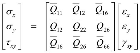
A composite material is not isotropic and therefore its stresses and strains cannot be related by the simple Hooke’s Law ( ). This law has to be extended to two-dimensions and redefined for the local and global co-ordinate systems [2]. The result is Equations (1) and (2).

Figure 1. Global co-ordinate system in relation to local co-ordinate system.
 (1)
(1)
 (2)
(2)
where σ1,2 are the normal stresses in directions 1 and 2; τ12 is the shear stress in the 1-2 plane; ε1,2 are the normal strains in directions 1 and 2; γ12 is the shear strain in the 1-2 plane; [Q] is the reduced stiffness matrix; σx,y are the normal stresses in directions x and y; τxy is the shear stress in the x-y plane; εx,y are the normal strains in directions x and y; γxy is the shear strain in the x-y plane; [ ] is the transformed reduced stiffness matrix.
The elements of the [Q] matrix in Equation (1) are dependent on the material constants and may be calculated using Equation (3).
 (3)
(3)
where E1,2 are Young’s modulus in directions 1 and 2; G12 is the shear modulus in the 1-2 plane; ν12,21 are Poisson’s ratios in the 1-2 and 2-1 planes.
The [ ] matrix in Equation (2) may be determined by Equation (4).
 (4)
(4)
where [T] is the transformation matrix; [R] is the Reuter matrix. These matrices are given by:
 (5)
(5)
where c = cosθ; s = sinθ.
The local stresses and strains in Equation (1) are related to the global stresses and strains in Equation (2) by Equation (6).
 (6)
(6)
Equations (1) to (6) are used to determine the stresses and strains for a single composite layer. Since composites are multi-layered entities, equations for this case must also be set up. The result is Equation (7).
 (7)
(7)
where N is the vector of resultant forces; M is the vector of resultant moments; ε0 is the vector of the mid-plane strains; κ is the vector of mid-plane curvatures. Vectors ε and κ are related to the global co-ordinates by Equation (8).
 (8)
(8)
where z is an arbitrary distance from the mid-plane.
The [A], [B], and [D] matrices in Equation (7) are known as the extensional, coupling, and bending stiffness matrices, respectively. The elements of these matrices may be determined from Equations (9) to (11).
 (9)
(9)
 (10)
(10)
 (11)
(11)
where n is the number of layers;  is the i-thj-th element of the [
 ] matrix of the k-th layer; hk is the distance of the top or bottom of the k-th layer from the mid-plane of the composite. Figure 2 illustrates how to determine the distance hk from the mid-plane.
The final aspect involved in the design of a composite structure is the failure analysis. There are various failure theories; however, the Tsai-Wu failure criterion is only one that closely correlates with experimental data. This failure theory is given by Equation (12).
 (12)
(12)
The parameters for the Tsai-Wu failure criterion are given by Equation (13).
 (13)
(13)
where  are the ultimate tensile stresses in direction 1 and 2;
  are the ultimate compressive stresses in direction 1 and 2;
  is the ultimate shear stress in the 1-2 plane.
In order to better facilitate the use of this failure theory, each stress component of Equation (12) was multiplied by a variable [2]. This variable is referred to as the strength ratio (SR) and combining this in Equation (12) resulted in Equation (14).
 (14)
(14)
The purpose of SR is to directly determine by what ratio the local stresses must be increased or decreased to avoid failure. This also directly relates to the applied forces. The criterion for SR is that it can only be positive. If SR is less than 1, then failure occurs because it means that the loading needs to decrease to avoid failure. A SR value of 1 implies that the composite structure is perfectly suited for the applied loading conditions. A value of greater than 1 means that the structure is more than capable of carrying the applied loading and that the loading may also be increased. For example, a SR value of 1.5 means that the loading may be increased up to 50% without failure occurring.

Figure 2. Locations of layers in a composite structure [2].
3. Programming
3.1. Conventional Approach Program
This approach follows the commonly found methods laid out in the various texts [2-4]. As stated above, the material constants, material limits, number of fibre layers, fibre angle of each layer, and the thickness of each layer as well as the loading conditions need to be known. The following procedure illustrates the steps involved in this approach:
1) Calculate the [Q] matrix for each layer using Equation (3).
2) Using Equation (5), compute the [T] matrix for each layer.
3) Determine [ ] matrix for each layer via Equation (4).
4) Find the location of the top and bottom surface of each layer, hk (k = 1 to n).
5) Use Equations (9), (10) and (11) to calculate the [A], [B], and [D] matrices.
6) Substitute these matrices as well as the applied loading into Equation (7) and solve the six simultaneous equations to determine the mid-plane strains (ε0) and curvatures (κ).
7) Find the global strains and stresses in each layer using Equations (8) and (2), respectively.
8) Find the local strains and stresses for each layer by using Equation (6).
9) Determine the parameters for the Tsai-Wu failure criterion via Equation (13).
10) Using these parameters and the local stresses for each layer, find SR via Equation (14).
Once SR has been determined, the designer will know whether the structure will fail or not. If failure occurs, the fibre angles and possibly the number of layers have to be adjusted, and the above procedure needs to be repeated until no failure takes place. Manual calculations would take a long period, therefore a program was written to perform the necessary calculations.
The program prompts the user for the following inputs:
• the material properties (E1, E2, G12 and ν12)
• the material limits ( ,
,  ,
,  ,
,  ,
, )
)
• the number of layers (N)
• the fibre angle (θ) of each layer
• the thickness (t) of each layer
• applied loading conditions
These input parameters were used to determine the [Q], [T], and [ ] matrices for each layer. All data concerning each layer (E1, E2, G12, ν12, θ, t, [Q], [T], and [
 ]) were stored in an array. The data in this array was used to calculate the [A], [B], and [D] matrices. Using these matrices and the applied loading conditions, the global and local stresses and strains were computed. The local stresses were compared to the material limits, via the Tsai-Wu failure criterion, to determine whether the composite will fail.
The computation of the various matrices and other relevant data was each carried out in a separate function. This means there was one function to determine the [Q] matrix, another to calculate the [T] matrix, and so on. A script file was written that controlled the use of each function. The purpose of the functions was to enable easier programming in future.
This program was tested against manually calculated examples in the various texts [2,3] and the results were exactly comparable to the manual computations. In an example (Example 4.3) by Kaw [2], the stresses and strains in a graphite/epoxy composite laminate were examined. This laminate consisted of three layers, with fibre angles of 0°, 30° and –45°, and each layer had a thickness of 5 mm. The material properties, material limits and loading conditions used in this example are given in Table 1.
The resulting global strains, global stresses, local strains and local stresses at the top, middle and bottom of each layer are shown in Figures 3 to 6, respectively.
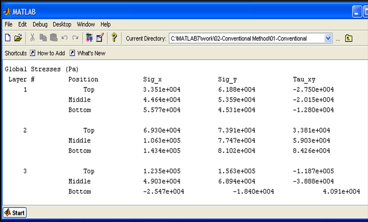
The values in Table 1 and the fibre angles of 0°, 30° and –45° were used as inputs in the Conventional Approach script file. The global and local stresses and strains were computed and are shown in Figures 7 to 10. The values in these tables and the ones in Figures 3 to 6 are exactly comparable. The conclusion from this is that the Conventional Approach program can accurately determine the stresses and strains in a flat unidirectional composite structure.
The Conventional Approach script file was further extended to include failure analysis via the Tsai-Wu failure theory. The resulting SR values for the top, middle and bottom of each layer is shown in Figure 11. The rows represent the layers and columns 1 to 3 represent the top, middle and bottom of each layer, respectively.
The SR values in Figure 11 indicate that the composite structure will fail first on layer 1 (SR = 0.6147) and then layer 2 (SR = 0.8870). It is clear from this that the input angles and number of layers were insufficient to carry the applied loads.
Although this program performs all the relevant calculations easily and automatically, and signifi-cantly shortens the design process, using the program to design a composite structure would require much guesswork. The designer would enter the necessary input values, allow the program to perform the various calculations, and then discover whether the composite structure would fail. If failure does occur, as in the above case, the designer may have to change the fibre angles and/or the thickness of each layer and/or the number of layers. The choice of values may be uncertain and values would have to be assumed. Furthermore, it would also be an uncertainty on which values to change. Much time may be spent in achieving a structure that would not fail. On the other hand, if failure does not occur, the structure may prove to be overdesigned in which case the manufacturing costs of the structure may increase as unnecessary material will be used. To overcome these problems, a new script file was generated.
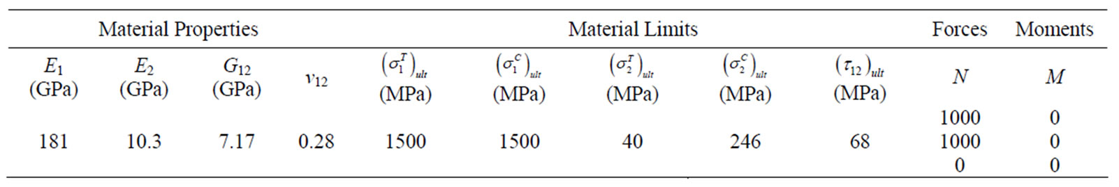
Table 1. Material properties, limits and loading conditions for graphi-te/epoxy composite example in Kaw [2].

Figure 3. Table from example in Kaw [2] showing global strains.

Figure 4. Table from example in Kaw [2] showing global stresses.

Figure 5. Table from example in Kaw [2] showing local strains.

Figure 6. Table from example in Kaw [2] showing local stresses.


3.2. Fibre-Angle-Output Program
Initially it was decided that this program should take the applied loading conditions, material properties and material limits as inputs. The program was to assume that the number of layers equals the number of input forces, and that the fibre angle of each layer equals the direction of each force. It would then perform all the necessary matrix calculations as in the Conventional Approach. The global and local stresses and strains would be determined as before and failure analysis with the Tsai-Wu criterion may be performed.
However, the assumptions made above cannot be used in a real situation as it may result in an overdesign of a composite structure as in the case of the conventional approach. Hence a program was written that does not make any assumptions but rather builds the laminate up one layer at a time. Basically this program varies the fibre angles to achieve a composite structure that is perfectly suited to carry the applied loading conditions. The

outputs of the program are the number of layers and the fibre angle of each layer.
The program asks the user to input the following:
• material properties
• material limits
• loading conditions
The [Q] matrix and the Tsai-Wu parameters can be calculated immediately as these do not vary with fibre angle but rather with material properties and limits. The program begins with one layer at an angle of 0° and computes hk, as well as the [T], [ ], [A], [B] and [D] matrices. Thereafter the mid-plane strains and curvatures, and, the global and local stresses and strains are calculated. The Tsai-Wu failure theory is applied and a value for SR is obtained for each layer.
The program then analyzes the SR values and confirms whether it is in a certain range. The lower limit of this range is 1 as any value below this would mean failure. The upper limit in this range is 1.2 and this is to avoid overdesigning.
If the SR value for each layer is between 1 and 1.2, then the design of the composite structure is complete. On the other hand, if the SR value for any of the layers is out of this range, the program varies that particular fibre angle to obtain a SR value between 1 and 1.2. However, due to the angle change all the matrix calculations have to be redone. A new SR value is obtained for each layer and this is compared to the old values. If the new SR value for a particular layer is higher than the old SR value, then the angle of that layer is changed to the new one. For example, after the initial calculation a layer with fibre angle of 30° has a SR value of 0.8. This is not acceptable and the program changes the angle to obtain a better SR value. Say at 35° the SR value is 0.9, the program will then change the angle of the 30° layer to 35°. If at 35° the SR value was 0.7, then the program will retain the 30° angle.
The program continues to change angles and compare old and new SR values until the SR value of each layer is between 1 and 1.2, in which case the design is completed. However, if this range cannot be achieved, a new layer is added on. The program starts from the beginning and recalculates the various matrices. SR values are obtained and the comparison between new and old values resumes. New layers will be added on until the SR value for each layer is between 1 and 1.2. The program then outputs the number of layers and the fibre angle of each layer. Figure 12 illustrates the procedure the script file follows to obtain the desired outputs.
The Fibre-Angle-Output program was subjected to several runs. The results, namely the number of layers and the fibre angles, needed to be verified. Therefore these were used as inputs in the Conventional Approach program. The Tsai-Wu failure theory was used and in each case there was no failure. As an example, consider the graphite/epoxy composite laminate examined earlier. The material properties, material limits and loading conditions for this laminate were given in Table 1. The SR values for three layers with fibre angles of 0°, 30° and –45° were shown in Figure 11. The values in Table 1

Figure 12. Flowchart describing the Fibre-Angle-Output program.
were input into the Fibre-Angle-Output program. The output of the program is shown in Figure 13.
It can be seen from Figure 13 that the number of layers is the same as when the example was analysed by the Conventional Approach program; however, the fibre angles are different. Here the required angles are 49°, –79° and 49° instead of the previous 0°, 30° and –45°. Further the SR values are all between 1 and 1.2 indicating no failure or overdesign.
The new fibre angles (49°, –79° and 49°) along with the material properties, material limits and loading conditions in Table 1 were then input into the Conventional Approach program. The resulting SR values were exactly the same as in Figure 13. Further, the local stresses of the new laminate, shown in Figure 14, was compared with the local stresses of the earlier laminate, shown in Figure 10. It can be seen that the local stresses in Figure 14 are constant through the thickness of each layer. This shows that the stresses were evenly distributed and not varied through the thickness of each layer.
Previously the SR value on the first layer was less than 1 (Figure 11) and lower than the other two layers indicating earliest failure. However with the new layup, the SR value has increased to a value greater than one. This means that the first layer is now capable of carrying a higher load and this is evident by the values for the local stresses. The previous value at the top of the first layer was 33.5 MPa (Figure 10), and the new value is 75.7 MPa (Figure 14). This clearly demonstrates the higher load bearing capability of the new laminate. Similar trends may be seen from the other positions and from the other two layers.


Figure 14. Local stresses for laminate with angles of 49°, –79°, and 49°.
It was then decided to increase the loading conditions of the 49°, –79° and 49° laminate to determine whether an increase in load will result in failure. The applied loads were increased by 10% and the resulting SR values are shown in Figure 15. It can clearly be seen that all the SR values for all the layers were less than 1. An increase in loading resulted in failure and therefore it may be deduced that the Fibre-Angle-Output program optimally designed the composite laminate for the loading conditions in Table 1. This further implies a saving in material cost as there would be no extra material used because of overdesigning.

Figure 15. SR ratios for 49°, –79° and 49° laminate with 10% increase in loading.
3.3. Finite Element Analysis
For further verification of the computational results, it was decided to perform finite element analyses on the laminates examined in the Conventional Approach program and the Fibre-Angle-Output program. The package used for the analysis was MSC Patran/Nastran 2007.
Two finite element models were setup, and both models represented a flat composite plate with material properties, material limits and loading conditions from Table 1. The first model had the same fibre layup that was used in the example for the Conventional Approach program, that is, 0°, 30°, and –45°. The analysis was run and the resulting fringe plots of the stress components of each layer were plotted. These plots are shown in Figure 16.
The stress plots from the finite element package corresponds to the local stresses experienced by a laminate, in particular the stresses occurring at the middle of each layer. Comparing the stress values in Figure 16 with the stresses incurred at the middle of each layer in either Figure 6 or Figure 10, it can be seen that the values are exactly the same. This implies that the model was correctly setup and that it may be used to evaluate local stresses of laminates designed with the Fibre-AngleOutput program.
The second model was setup and was similar to the first model in every aspect except for the fibre layup. This model had the new fibre layup (49°, –79°, and 49°) that was determined by the Fibre-Angle-Output program. The fringe plots of the stress components from this analysis are shown in Figure 17. Here it is also evident that the values in the plots exactly correspond to the stress values at the middle of each layer in Figure 14. This verifies the above results from the Fibre-AngleOutput program and supports the conclusion that the program optimally designed the composite laminate, with the fibre layup of 49°, –79° and 49°, for the loading conditions in Table 1.
4. Conclusions
A MATLAB script file was generated that uses the conventional approach in the design of composite laminates. The inputs are the material properties, material limits, number of fibre layers, and the fibre orientation and thickness of each layer as well as the loading conditions. These values are then used in the governing equations, based on Hooke’s law for two-dimensional unidirectional laminates, to determine the global and local stresses and strains. The local stresses are compared to allowable limits via the Tsai-Wu failure theory. The results from this program were compared to manually calculated examples in the various texts [2,3] and it was found that they were exactly comparable.
The above program required much guesswork in choosing inputs and was therefore inadequate to design composite laminates. Hence it was adapted to take material properties, material limits and the loading conditions as inputs. The necessary calculations were performed and the optimum number of fibre layers required as well

Figure 16. Fringe plots from Patran showing stress components for 0°, 30°, and –45° laminate.

Figure 17. Fringe plots from Patran showing stress components for 49°, –79°, and 49° laminate.
as the fibre angle of each layer was determined. These outputs were input into the Conventional Approach program in order to verify the results. In each case the resulting composite structure did not fail. The example used showed that the Fibre-Angle-Output program optimally designed the composite laminate for the given loading conditions. Finite element analyses were conducted to verify this conclusion.
The use of these programs will greatly reduce the design time of composite structures as the numerous computations are completed in a fraction of the time that it would take if done manually. The designer merely has to run the Fibre-Angle-Output program, and view the number of layers required and the fibre angle for each layer. The program will also aid in reducing material costs. Presently the program is limited to flat unidirectional structures but work is underway to extend it to three dimensions. There is no limit on the type of composite material as far as the matrix and fibre reinforcement is concerned.
5. REFERENCES
- S. K. Mazumdar, “Composite Manufacturing: Materials, Product, and Process Engineering,” CRC Press LLC, Boca Raton, 2002.
- A. K. Kaw, “Mechanics of Composite Materials,” CRC Press LLC, Boca Raton, 1997.
- C. T. Herakovich, “Mechanics of Fibrous Materials,” John Wiley & Sons Inc., Hoboken, 1998.
- R. M. Christensen, “Mechanics of Composite Materials,” Dover Publications, New York, 2005.
- M. Akbulut and F. O. Sonmez, “Optimum Design of Composite Laminates for Minimum Thickness,” Computers and Structures, Vol. 86, No. 21-22, 2008, pp. 1974-1982.
- K. Sivakumar, N. G. R. Iyengar and K. Deb, “Optimum Design of Laminated Composite Plates with Cutouts Using a Genetic Algorithm,” Composite Structures, Vol. 42, No. 3, 1998, pp. 265-279.
- S. A. Barakat and G. A. Abu-Farsakh, “The Use of an Energy-Based Criterion to Determine Optimum Configurations of Fibrous Composites,” Composite Science and Technology, Vol. 59, No. 12, 1999, pp. 1891-1899.
- P. Kere, M. Lyly and J. Koski, “Using Multicriterion Optimization for Strength Design of Composite Laminates,” Composite Structures, Vol. 62, No. 3-4, 2003, pp. 329-333.
- C. H. Park, W. I. Lee, W. S. Han and A. Vautrin, “Weight Minimization of Composite Laminated Plates with Multiple Constraints,” Composite Science and Technology, Vol. 63, No. 7, 2003, pp. 1015-1026.
- MediaWiki, “MATLAB,” 2008. http://en.wikipedia.org/ wiki/MATLAB
- R. V. Dukkipati, “MATLAB for Mechanical Engineers,” New Age International (P) Limited, New Delhi, 2008.
- G. Z. Voyiadjis and P. I. Kattan, “Mechanics of Composite Materials with MATLAB,” Springer Netherlands, Dordrecht, 2005.
- A. Gilat, “MATLAB: An Introduction with Applications,” John Wiley & Sons Inc., Hoboken, 2008.
- B. D. Hahn and D. T. Valentine, “Essential MATLAB for Engineers and Scientists,” Butterworth-Heinemann, Rome, 2007.