Journal of Signal and Information Processing, 2011, 2, 253-256
doi:10.4236/jsip.2011.24035 Published Online November 2011 (http://www.SciRP.org/journal/jsip)
1
New Formulas for Irregular Sampling of
Two-Bands Signals
Bernard Lacaze
Telecommunications for Space and Aeronautics, Toulouse, France.
Received March 15th, 2011; revised June 20th, 2011; accepted June 30th, 2011.
ABSTRACT
Many sampling formulas are available for processes in baseband


,aa at the Nyquist rate πa. However signals
of telecommunications have power spectra which occupate two bands or more. We know that PNS (periodic
non-uniform sampling) allow an errorless reconstruction at rate smaller than the Nyquist one. For instance PNS2 can
be used in the two-bands case at the Landau rate

,ab ba

,


πab We prove a set of formulas which are
available in cases more general than the PNS2. They take into account two sampling sequences which can be periodic
or not and with same mean rate or not.
Keywords: Stationary Process e s , Irregular Sampling, Two-Bands Processes
1. Introduction
Communications signals are often transmitted in frequ-
ency channels which are in the form where the
width is small with respect to . For instance
we have for the whole FM band (87.5
MHz, 108 MHz). Of course, the occupied frequency in-
terval by a single station is smaller which leads to rela-
tive occupency very weak. When modelling by stationary
processes, negative frequencies are taken into account.
Real processes are transmitted in frequency bands in the
form . We know that such processes
can be reconstructed by sampling at the Landau rate

,ba
a


2

abab

,ab


/0.a

,ba

2πab , which is weaker than the Nyquist rate
2πa [1]. PNS2 (Periodic Nonuniform Sampling of
order 2) is the most known example [2,3]. In the case of
baseband signals where power spectra are strictly in
, any sampling plan regular enough can be asso-
ciated with errorless formulas provided that the sampling
rate is larger than

,aa

2πa [4-6]. They are close to La-
grange interpolation formulas, replacing far samples by
well-chosen sequences. However this kind of scheme
cannot be used when power spectra are not in baseband.
This paper addresses the problem of errorless sampling
of stationary processes Z =




,Zt t with spectral
support inside two symmetric sets of the real line. For
instance and without loss of generality, let this support be
(1), where l

 and >0

. This means that [7,8]




E=e
iZ
ZtZ ts



d







 (2)
where E


.. stands for the mathematical expectation (or
ensemble mean) and the superscript  for the complex
conjugate.


Z
s

is the spectral density of the process
Z. We assume that


=0
Z
s 
in some neighboorhood
of the bounds of 0

to be sure that Z is oversampled
with respect to the Landau's theorem in all studied cases.
Knowing that

is arbitrary the minimal sampling
rate for errorless reconstruction is 2 because 0=4π
[1]. Samplings like PNSn (periodic nonuniform sam-
pling of order n) may be solutions of the problem [9],
[10]. For example we have the formula [2,3]




 


sin 2πsin 2π
=sin 2π
ab
Utltb Utlat
Zt la b


 (3)





sin π
=π
xn
txn
Ut Znx
txn

 



provided that


2la b

. We are in the case of a PNS2
where the sampling sequences are and
ab

.












=21π,21π21π,2 1πll ll


   
(1)

New Formulas for Irregular Sampling of Two-Bands Signals
254
In this paper we highlight a class of sampling sequ-
ences which answer the problem, and we give the associ-
ated reconstruction formulas. They generalize the PNS2
sampling set properties (and more generally the PNSn
sets properties).
2. A Sampling Formula
Let Z

=, ,=1,2
jj
n
tn jt
be two sampling sequences with distinct elements
( whatever ) such that:
12
nm
tt,mn
1) It exists two sampling formulas for the process in
baseband of width 2 defined by two kernels π


1,
g
tx
and

2,
g
tx:


 
=, ,=1
=0 forπ,π
jj
jn n
n
Z
Ztg ttZtj
s
,2






 




(4)
for some >0

.
2) It exists two real numbers 12
,

 such that for all
n
21
2,
j
nj
lt    . (5) 
At these conditions, and when (

 is defined by (1))

=0,
Z
s

 
we have the sampling formula (6).
The proof is in Appendix 1.
3. Examples
3.1. Example 1
The well-known formula (3) for the PNS2 verifies (6)
with (sinc=
x
sin
x
x)




12
12
1
1
1
2
=2 ,=2 ,==2
,=sincπ
,=sincπ.
nn
n
n
lalb kknl
gtt tan
gtt tbn








3.2. Example 2
Let consider the following sampling scheme
12 2
221
11
=,=2,=2,0< <
22
nn n
tntnatnaa


(6) is available with [11,12],





 

 
122
12221
1
1
2
22
2
221
=0, =2,=2,=4,=41
,=sincπ
π1π
,=12sinsinc 2
222
ππ 1
,=12sin sinc2
22
nnn
n
n
n
n
n
knllaknlknl
gtt tn
2
g
ttt at an
gtttata n






















Actually we are in the PNS4 frame with sequences based
on 1
2,2,2,2 1,
2
nnanan n

.
3.3. Example 3
We assume that
12 12 21
= ,=,0,,,...,
22 2
nn nnl
tntnabb ll l


 


with 2πla

 and the n constant for b>1nN
(for instance equal to 0). We are no longer in the PNS
frame (except when all are equal). We can take
n
b


12
12
1
1
=0,=2,=2 ,=22
,=sincπ
nn
n
knl laknlb
gtt tn






n
l
where


2
2,n
g
tt is given by (7) (see the Appendix 2)
with

0
1
1=.
1
bn
n
z
na
Fz z
nab











 (8)
If is large and then if the increments l1l are small,
.
  
 
 
12 11 2
1
12
22 1
2
21
1
=1,sin2π
sin π
,sin2π
=2,and
kk
nn nn n
n
nn n
jjj
jnnn

Z
tgttZt
gttZt ltt
ltkk












 






ltt
(6)

 




2
2
1,0
sin π
,= sinπ
1,=0.
n
n
'
nnn
nn
n
b
tanbFnab b
gtt Ftta
b
tanFna 


 





(7)

New Formulas for Irregular Sampling of Two-Bands Signals255
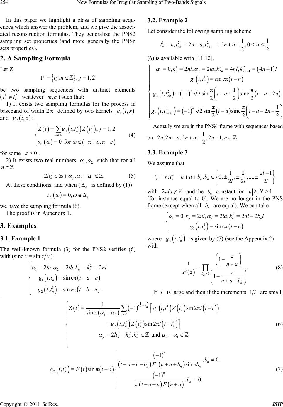
we have a model for (observed) jitter quantified at the
value 1l. Of course, we can complicate the sampling
plan by introducing sampling gaps in the .
1
n
t
3.4. Example 4
Examples above deal with two samplings t1 and t2 with
equal mean rate 1. Following the value of (the place
of subbands) we can imagine samplings with mean rates
which are different and not multiple (but rational be-
tween them). For instance consider the following case
l
12
2
=, =,3,2.
3
nn
n
tntalla 
This corresponds to



12
12
1
1
2
2
4
=0,=2,=2 ,=3
,=sincπ
3π2
,=sinc
23
nn
n
n
knllakn
gtt tn
n
gtt ta











l
 
2
2,n
g
tt is the usual sampling formula matched to the
sampling rate 3/2 delayed by , true for power spectra
in
a

3π2,3π2.

The larger the better the choice
for available samplings. Unlike the preceeding examples,
we are in a situation of a true oversampling (
l

is arbi-
trarily small). However, if is not too small, the mean
rate sampling is more favourable than the Nyquist one.
l
3.5. Example 5
One or both sequences can be mixed. For instance
12
for even
=,=,2,2
3for odd
4
nn
nn
ttnal
nn

 



 .la
The formula (6) can be used when ,
with
2,2lla






11 2
12 212
1
1
2
2
3
=0,=4,=21,=2,=2
2
2for even
πcosπ6
π2π
,=sincos 3
23 for odd
πcos π8
,=sincπ
nn n
n
n
knlk lnlakn
n
tn n
tt
gtt
n
tn n
gtt tna


















l
0
4. Conclusions
Most of the time, processes used in communications occ-
py symmetrical power spectral bands in the form u

=, ,,>ba aba

. Very often, the relative ban-
dwidth 2bab is small. However, most of the sam-
pling formulae are matched to baseband processes where


=,aa . In this case the choice of errorless samplings
is large, whatever the sampling, uniform or irregular [5,6,
13]. The sampling mean rate for errorless reconstruction is
πa in the latter case (the Nyquist rate) and it is


πba in the former case (the Landau rate) [1]. In
communications the Landau rate is small in front of the
Nyquist rate. The research for errorless samplings with
Landau rate is important for reducing calculus cost. The
choice of errorless samplings is limited to the PNS [9,10]
and has to be increased. It is the aim of this short paper. A
new sampling formula is proved and examples are given.
They are based on formulas true in baseband and generally
well-known [4,14,15]. Example 3 deals with irregular
samplings at the Landau rate and can be used in the pres-
ence of jitter. In example 4, we have two samplings with
different periods which generalizes the PNS2. The method
which is used can be generalized to other power spectra
including more than two pieces [16,17]. It is also possible
to use a mixing of several periodic samplings for the se-
quences t1 and/or t2 [11,12].
REFERENCES
[1] H. J. Landau, “Sampling, Data Transmission, and the
Nyquist Rate,” Proceedings of the IEEE, Vol. 55, No. 10,
1967, pp. 1701-1706. doi:10.1109/PROC.1967.5962
[2] B. Lacaze, “About Bi-Periodic Samplings,” Sampling Th-
eory in Signal and Image Processing, Vol. 8, No. 3, 2009,
pp. 287-306.
[3] B. Lacaze, “Equivalent Circuits for the PNS2 Sampling
Scheme,” IEEE Circuits and Systems, Vol. 57, No. 11,
2010, pp. 2904-2914. doi:10.1109/TCSI.2010.2050228
[4] A. J. Jerri, “The Shannon Sampling Theorem. Its Various
Extensions and Applications. A Tutorial Review,” Pro-
ceedings of the IEEE, Vol. 65, No. 11, 1977, pp. 1565-
1596. doi:10.1109/PROC.1977.10771
[5] B. Lacaze, “Reconstruction Formula for Irregular Sam-
pling,” Sampling Theory in Signal and Image Processing,
Vol. 4, No. 1, 2005, pp. 33-43.
[6] B. Lacaze, “The Ghost Sampling Sequence Method,”
Sampling Theory in Signal and Image Processing, Vol. 8,
No. 1, 2009, pp. 13-21.
[7] H. Cramér and M. R. Leadbetter, “Stationary and Related
Stochastic Processes,” Wiley, New York, 1966.
[8] A. Papoulis, “Signal Analysis,” McGraw Hill, New York,
1977.
[9] J. R. Higgins, “A Sampling Theorem for Irregular Sample
Points,” IEEE Transactions on Information Theory, Vol.
22, No. 5, 1976, pp. 621-622.
doi:10.1109/TIT.1976.1055596
[10] J. R. Higgins, “Some Gap Sampling Series for Multiband
Signals,” Signal Processing, Vol. 12, No. 3, 1987, pp. 313-
319. doi:10.1016/0165-1684(87)90100-9

New Formulas for Irregular Sampling of Two-Bands Signals
256
[11] J. L. Yen, “On Nonuniform Sampling of Bandwidth-
Limited Signals,” IRE Transactions on Circuit Theory,
Vol. 3, No. 4, 1956, pp. 251-257.
[12] B. Lacaze, “About a Multiperiodic Sampling Scheme,”
IEEE Signal Processing Letters, Vol. 6, No. 12, 1999, pp.
307-308. doi:10.1109/97.803430
[13] B. Lacaze, “A Theoretical Exposition of Stationary Proc-
esses Sampling,” Sampling Theory in Signal and Image
Processing, Vol. 4, No. 3, 2005, pp. 201-230.
[14] K. Seip, “An Irregular Sampling Theorem for Functions
Bandlimited in a Generalized Sense,” SIAM Journal on
Applied Mathematics, Vol. 47, No. 5, 1987, pp. 1112-
1116. doi:10.1137/0147073
[15] A. I. Zayed and P. L. Butzer, “Lagrange Interpolation and
Sampling Theorems,” In: F. Marvasti, Ed., Nonuniform
Sampling: Theory and Practice, Kluwer Academic, 2001,
pp. 123-168. doi:10.1007/978-1-4615-1229-5_3
[16] Y.-P. Lin and P. P. Vaidyanathan, “Periodically Nonuni-
form Sampling of Bandpass Signals,” IEEE Transactions
on Circuits and Systems II, Vol. 45, No. 3, 1998, pp. 340-
351.
[17] R. Venkataramani, “Perfect Reconstruction Formulas and
Bounds on Aliasing Error in Sub-Nyquist Nonuniform
Sampling of Multibands Signals,” IEEE Transactions on
Information Theory, Vol. 46, No. 6, 2000, pp. 2173-2183.
Appendix
Appendix 1
If


,= ,e
j
mit
mn
jj
nm
ht gtt



j
n
(4) is equivalent to
 
2 π
πe, d
lim it m
jZ
mht s





 
=0.

Then we also have


=e e,
j
iat
iatj j
n
j
nn
n
Z
tgtt




Zt
a
(9)
when
 
=0for π,π.
Z
sa

  
Now we assume that


=0
Z
s  for


 . We
write:
 
 

 
=
=0,21, 21
=0,21, 21.
Z
Z
ZtZ tZ t
sll
sl


l









 

 



.
(10)
We define (11)
From (9), (10) we have

 
2π2π
2π
,=e e
iilt
ilt j
j
A
tZtZ





t (12)
When
=2,,whatever
jjj
jnnn
ltkkn   
we have


 
π
,=e1 ,
j
ik.
j
j
jn
jj
nnn
A
tgt







tZt

(13)
The linear system (12,13) is solved in (14) which leads
to (6). We understand the key of this formula. The prob-
lem is to write (1) so that


j
n
j
n
Z
t
 and
Z
t

 disap-
pear (they are not observed) and the

j
Z
n
t appear (they
are observed).
Appendix 2
With


F
z defined by (8) we consider n
I
the com-
plex integral
  
e
=d
sin π
iz
nCn
I
z
ztFz za



where is the square crossing the axes Ox, Oy at the
points
n
C
=12,=1xna yn 2. Because


=<
lim
zFz

 
we also have for


π,π



 =0.
lim n
nI 
We apply the residue’s theorem with order 1 singulari-
ties at the points n nab

 with for =0
n
b>.nN
Consequently







=0
0
1e
e=
sin ππ
1e .
sin
nina
it
bn
ninab
n
'
bnn
n
Fttta nFn a
tanbFnab b









 

n
(15)
We obtain (7) from (15) using the fundamental isometry
which allows to change eix

by

Z
x in (15) [13].

 
2π2π
2π
,= ,ee
j
jiilt
ilt
jj
jn
n
jjn nn
n
Atg ttZ tZt






.
j










(11)
   
ππ
12
122 1
21
1
=,esinπ2,esinπ2
sin
=2 ,
ii
jjj
jnnn
Z
tAt ltAt
ltk k

 



 





lt
(14)