Natural Science
Vol.4 No.12(2012), Article ID:25556,13 pages DOI:10.4236/ns.2012.412132
Analytical expressions of steady-state concentrations of species in potentiometric and amperometric biosensor
![]()
1Department of Mathematics, Bharath Niketan Engineering College, Theni, India
2Department of Mathematics, The Madura College, Madurai, India; *Corresponding Author: raj_sms@rediffmail.com
Received 24 September 2012; revised 27 October 2012; accepted 10 November 2012
Keywords: Enzyme Electrodes; Enzyme Reactors; Potentiometry; Amperometry; Homotopy Analysis Method; Biosensor
ABSTRACT
A mathematical model of potentiometric and amperometric enzyme electrodes is discussed. The model is based on the system of non-linear steady-state coupled reaction diffusion equations for Michaelis-Menten formalism that describe the concentrations of substrate and product within the enzymatic layer. Analytical expressions for the concentration of substrate, product and corresponding flux response have been derived for all values of parameters using Homotopy analysis method. The obtained solution allow a full characterization of the response curves for only two kinetic parameters (The Michaelis constant and the ratio of overall reaction and the diffusion rates). A simple relation between the concentration of substrate and products for all values of parameter is also reported. All the analytical results are compared with simulation results (Scilab/Matlab program). The simulated results are agreed with the appropriate theories. The obtained theoretical results are valid for the whole solution domain.
1. INTRODUCTION
Theoretical models of enzyme electrodes give information about the mechanism and kinetics of the biosensor. The information gained from mathematical modeling can be useful in sensor design, optimization and predict tion of the electrode’s response. Enzyme-based systems, i.e. the combination of enzyme-reactor sensor and enzyme electrodes have gained considerably more importance for chemical analysis and also for clinical diagnostics [1,2]. Blaedel et al. [3] have derived explicit solution of electrodes for steady-state conditions which can apply to very high substrate concentration or to sufficiently low substrate concentration. Guilbault and Nagy [4] proposed an approximation which is used for sensors with very thin enzyme membranes in contact with diluted substrate samples. Hameka and Rechnitz [5] have used Laplace transforms to treat potentiometric enzyme electrodes. Tranh-Minh and Broun [6] also solved the differential equations for reaction and diffusion processes by using a numerical method. Morf [7,8] presented a relatively simple approach for the electrode response that applies to the whole range of substrate concentrations by obtaining an explicit result. Glab et al. [9-11] extended this theory to account for additional influence arising from the presence of pH-buffering systems. Mell and Maloy [12,13] have obtained the current response as a function of time and substrate concentration using numerical simulation. Olesson et al. [14] treated the behavior of these sensors in flow-injection analysis applications. Albery and Bartlett [15] studied the steady-state current response of modified enzyme-based sensors where electron transfer from the enzyme to the electrode occurs directly by a redox mediator. Later these authors [16] have derived 11 equations to differentiate between 7 limiting cases by offering a complete theoretical treatment of the basic reaction and diffusion processes in homogeneous solution. Mackey et al. [17] recently studied the current efficiency of sensors with a monolayer of two enzymes.
Several groups [18-20] introduced numerical method for the study of amperometric and cyclic-voltammetric enzyme electrodes based on Michaelis-Menten kinetics. The available theoretical descriptions of enzyme electrodes seem to be quite complex. Reaction and diffusion processes in the enzyme layer are modeled by a finitedifference method [21-32]. Morf et al. [33] presented the theoretical model for an amperometric glucose sensor for low substrate concentration and high benzoquinone concentration compared with respective Michaelis constants. To my knowledge no rigorous analytical expression of concentration of substrate and mediator of ampereometric glucose sensor under steady-state conditions for all values of parameters have been reported. The purpose of this communication is to derive approximate analytical expressions for the steady-state concentrations and flux for all values of parameters α, β and γ using Homotopy analysis method. This dimensionless parameter are defined in the Eq.6.
2. MATHEMATICAL FORMULATION OF THE PROBLEM
In this paper we consider the analytical systems based on an enzyme-containing bulk membrane of thickness d that is contacted on one side with an aqueous solution of the substrate S (refer Figure 1).
The substrate molecules entering the membrane phase react according to a Michaelis-Menten type enzymecatalyzed reaction [31,32] to yield an electroactive product P. The corresponding governing equations in Cartesian coordinates for planar diffusion and reaction in a membrane may be written as follows [33,34]:
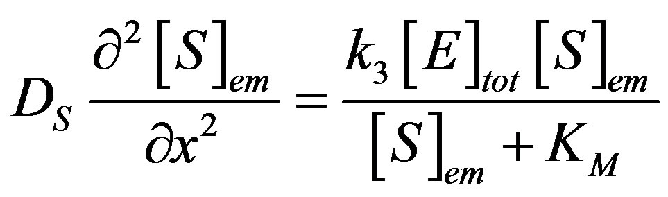 (1)
(1)
 (2)
(2)
where  and
and  are the concentrations of the species in the enzyme membrane, DS and DP are the corresponding diffusion coefficients,
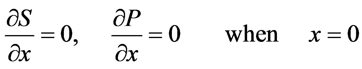
  is the total concentration of free enzymes and enzyme-substrate complexes that is assumed to be constant within the membrane including the surface zones, v is the number of product species obtained per substrate molecule, k3 is the rate constant for the irreversible step of product formation, and KM the Michaelis constant [31,32]. The Eqs.1 and 2 are solved for the following boundary conditions by assuming the zero fluxes at x = 0 and of equilibrium distribution at x = d [33,34].
 (3)
(3)
 (4)
(4)
For enzyme reactors, the outward flux of product species at x = d is described by:
 (5)
(5)
where JP is the outward flux of the product species and DP is the diffusion coefficient of the product.
3. DIMENSIONLESS FORM OF THE PROBLEM
To compare the analytical results with simulation results, we make the above non-linear partial differential equations Eqs.1 and 2 in dimensionless form by defining
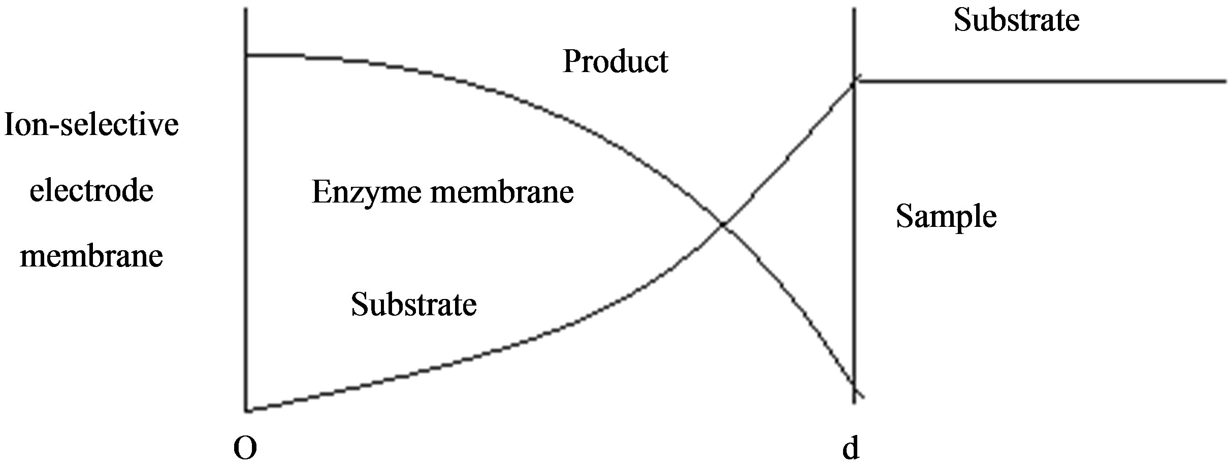 (a) Potentiomtric enzyme electrode
 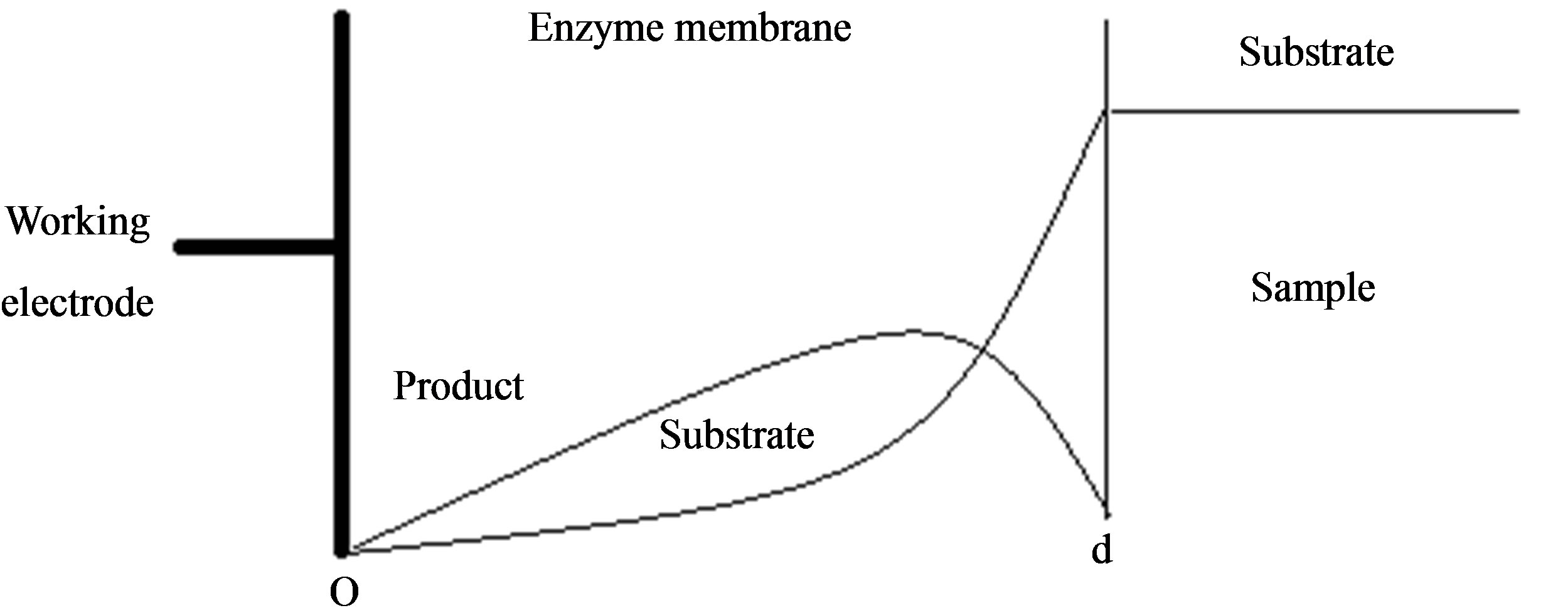 (b) Amperometric enzyme electrode
Figure 1. Various analytical scheme of enzyme-based system.
the following parameters:
 (6)
(6)
The Eqs.1 and 2 reduces to the following dimensionless form:
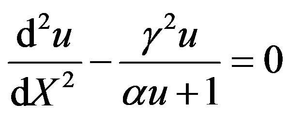 (7)
(7)
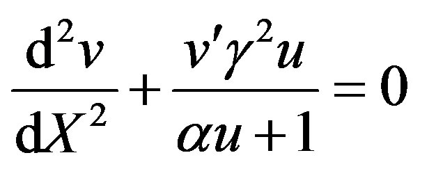 (8)
(8)
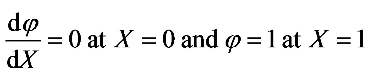
where u and v represents the dimensionless concentration of substrate and product. α and β are saturation parameter and γ is the reaction/diffusion parameter (Thiele modulus). Now the boundary conditions may be presented as follows [33,34]:
 (9)
(9)
 (10)
(10)
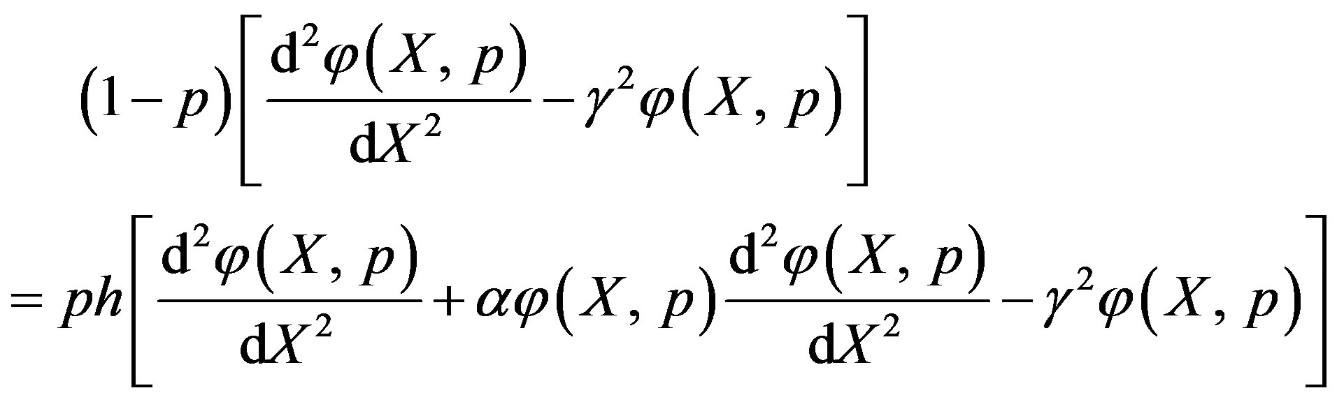
4. ANALYTICAL SOLUTIONS USING HOMOTOPY ANALYSIS METHOD
Recently, Homotopy analysis method (HAM) has been developed to solve different types of non-linear problems. Many problems of engineering and allied disciplines have been successfully solved [35,36]. The major advantages of this method are that it does not require the presence of small/large parameter unlike the perturbation method or delta decomposition method and can be applied to any type of nonlinearity. Further, working of HAM reduces to those of other methods for a certain choice of auxiliary quantities defined later [36,37], and it can easily be implemented in various symbolic soft computing tools e.g. MATHEMATICA, MAPLE etc. A details of this method can be found in the original work of Liao [36]. The Homotopy analysis method [38,39] was first proposed by Liao in 1992. The basic concept of Homotopy analysis method is given in [40]. By solving the above Eq.7 using HAM [38-44], we can obtain the concentration of substrate in dimensionless form as follows:
 (11)
(11)
Detailed derivation of the above Eq.11 is described in Appendix A. Adding the Eqs.7 and 8 we get
 (12)
(12)
Integrate the above Eq.12 twice and using the boundary conditions (9) and (10), we can obtain the concentration of product as follows:
 (13)
(13)
The normalized flux becomes,
 (14)
(14)
The above equation represent the dimensional flux for all values of parameter for steady state conditions.
5. LIMITING CASES
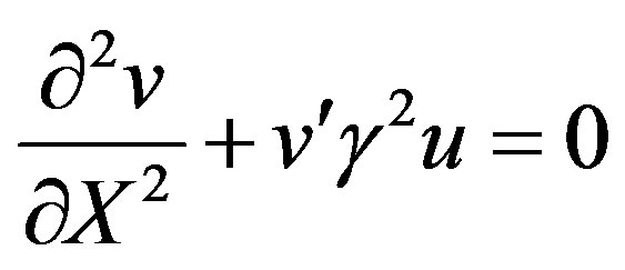
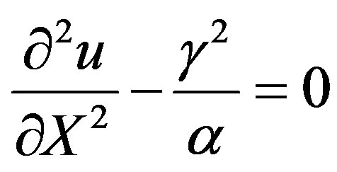
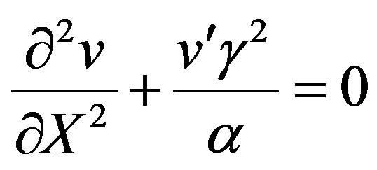
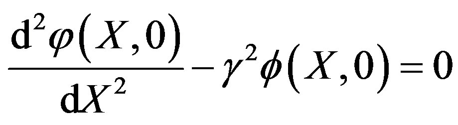
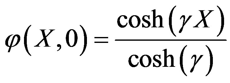
5.1. Limiting Case: 1-Unsaturated (First-Order) Catalytic Kinetics
We consider the situation when the substrate concentration is sufficiently low, that is for , the catalytic reaction follows first-order kinetics. This situation will pertain when the product
 . Hence Eqs.7 and 8 are reduces to
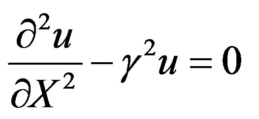 (15)
(15)
 (16)
(16)
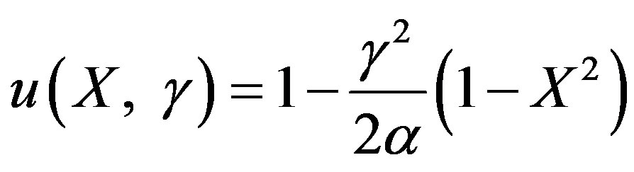
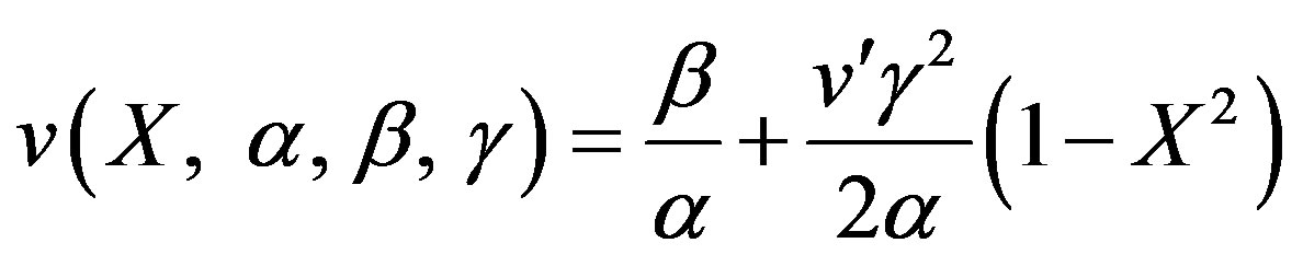
Hence the non-linear reaction/diffusion equation Eqs.7 and 8 has been reduced to the linear equation. Hence the concentration profiles of substrate and product are given by:
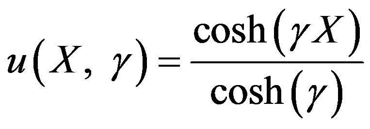 (17)
(17)
 (18)
(18)
In this case the dimensionless flux becomes
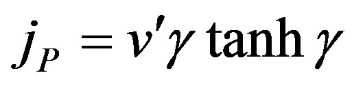 (19)
(19)
The Eqs.17 and 18 are same as Eqs.7 and 8 in [33].
5.2. Limiting Case: 2-Saturated (Zero-Order) Catalytic Kinetics
For very high substrate concentrations,  , the enzyme-catalyzed reaction becomes zero-order kinetics. In this case
  and Eqs.7 and 8 reduces to
 (20)
(20)
 (21)
(21)
Now the concentration of substrate and product becomes as follows:
 (22)
(22)
 (23)
(23)
The normalized flux is given by
 (24)
(24)
Recently Morf et al. [33] have derived the above (Eqs.22-24) same results (Eqs.14 and 15) in Ref. [33].
6. NUMERICAL SIMULATION
The two non-linear reaction/diffusion equations (Eqs.7 and 8) corresponding to the boundary conditions (Eqs.9 and 10) were solved by numerical methods. We have used pdex4 to solve these equations (Pdex4 in MATLAB is a function to solve the initial-boundary value problems of differential equations). The numerical solution is compared with our analytical results and is shown in Figures 2 and 3. Tables 1-4 illustrate the comparison of analytical result obtained in this work with the numerical result. The relative difference between numerical and analytical results are within 0.68% for all possible values of parameters considered in this work. A satisfactory agreement is noticed for various values of the Thiele modulus and possible small values of reaction/diffusion parameters.
7. DISCUSSION
7.1. Concentrations
The reaction diffussion parameter γ, is indicative of the competition between the reaction and diffusion in the matrix. When γ is small the kinetics dominate and the uptake of substrate is kinetically controlled. The overall kinetics are governed by the total amount of active enzyme, i.e. . When γ is large, diffusion limitations
 (a)
(a)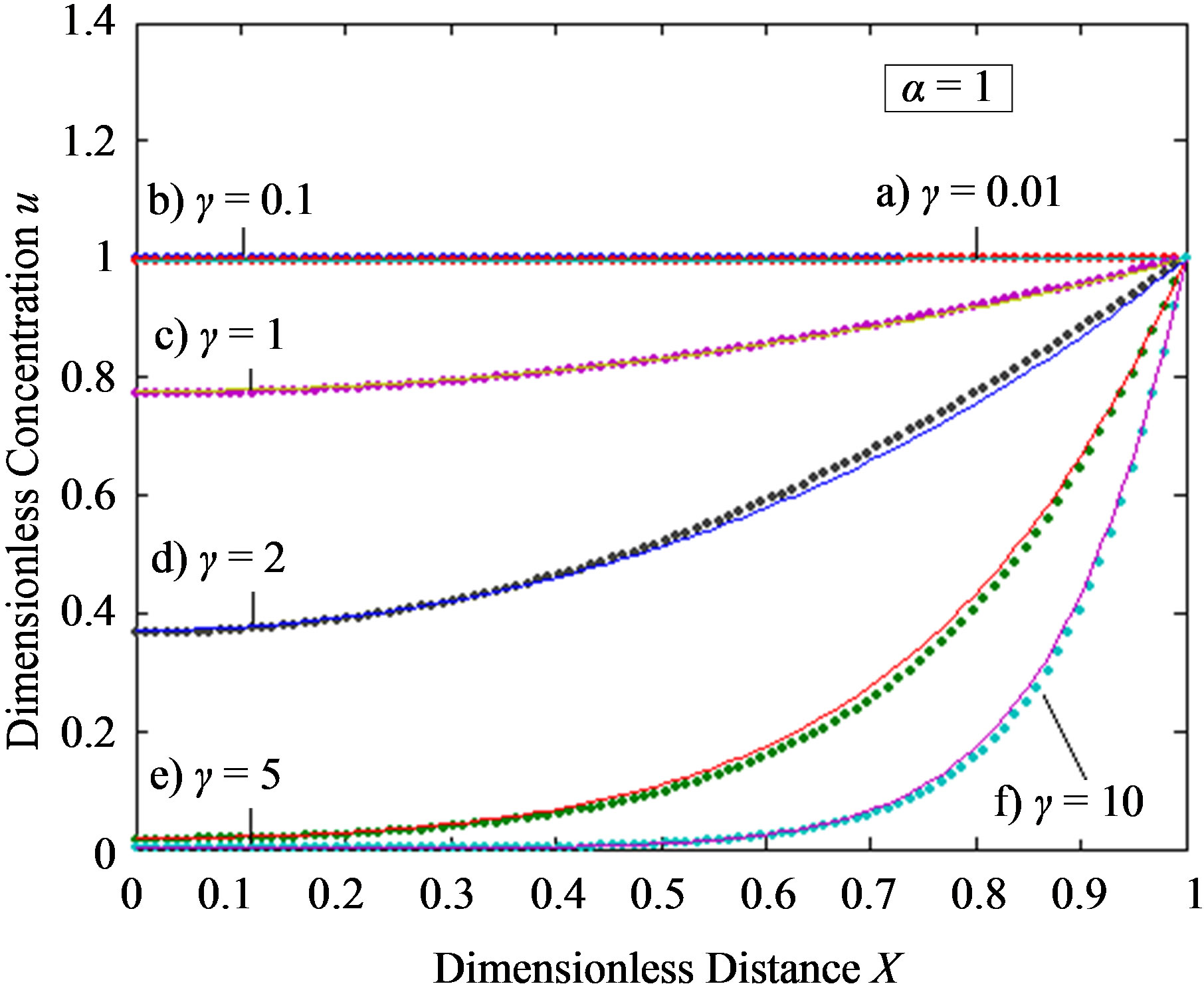 (b)
(b)
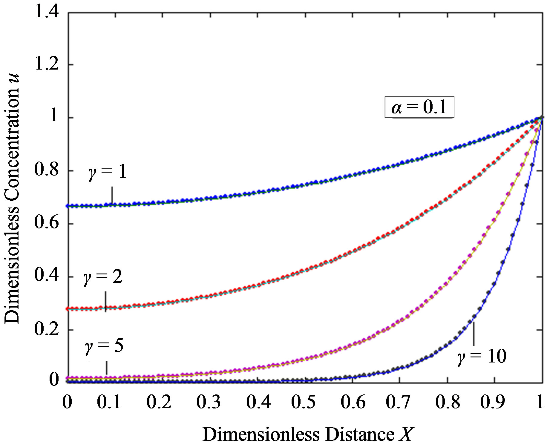
Figure 2. Dimensionless steady-state concentration profiles of the substrate u for various values of γ using the Eq.11. (a) The h value is –1; (b) a) b), e), f); h = –0. 5, c); h = –0. 7, d); h = –1. Solid lines represent the numerical simulation and the dotted lines represent the analytical solution.
are the principal determining factor. The concentration gradient near the electrode, and hence the flux of substrate to the electrode, decreases with an increase in γ. For a given layer, and hence value of γ, the concentration profile is also altered according to the bulk concentration of the substrate. Thus an increased substrate concentration causes a decrease in the flux to the electrode. Eqs.11 and 13 are the new and simple analytical expressions of concentrations of substrate and product respectively. The analytical expression of concentration of substrate, product and flux are summarized in Tables 5 and 6.
In Figures 2 and 3, the profiles of substrate as well as product concentration in the enzyme layer are presented. The normalized concentration of substrate is represented in Figures 2(a) and (b). From this Figure, it is evident that the value of substrate concentration S decreases
 (a) α = 0.01
 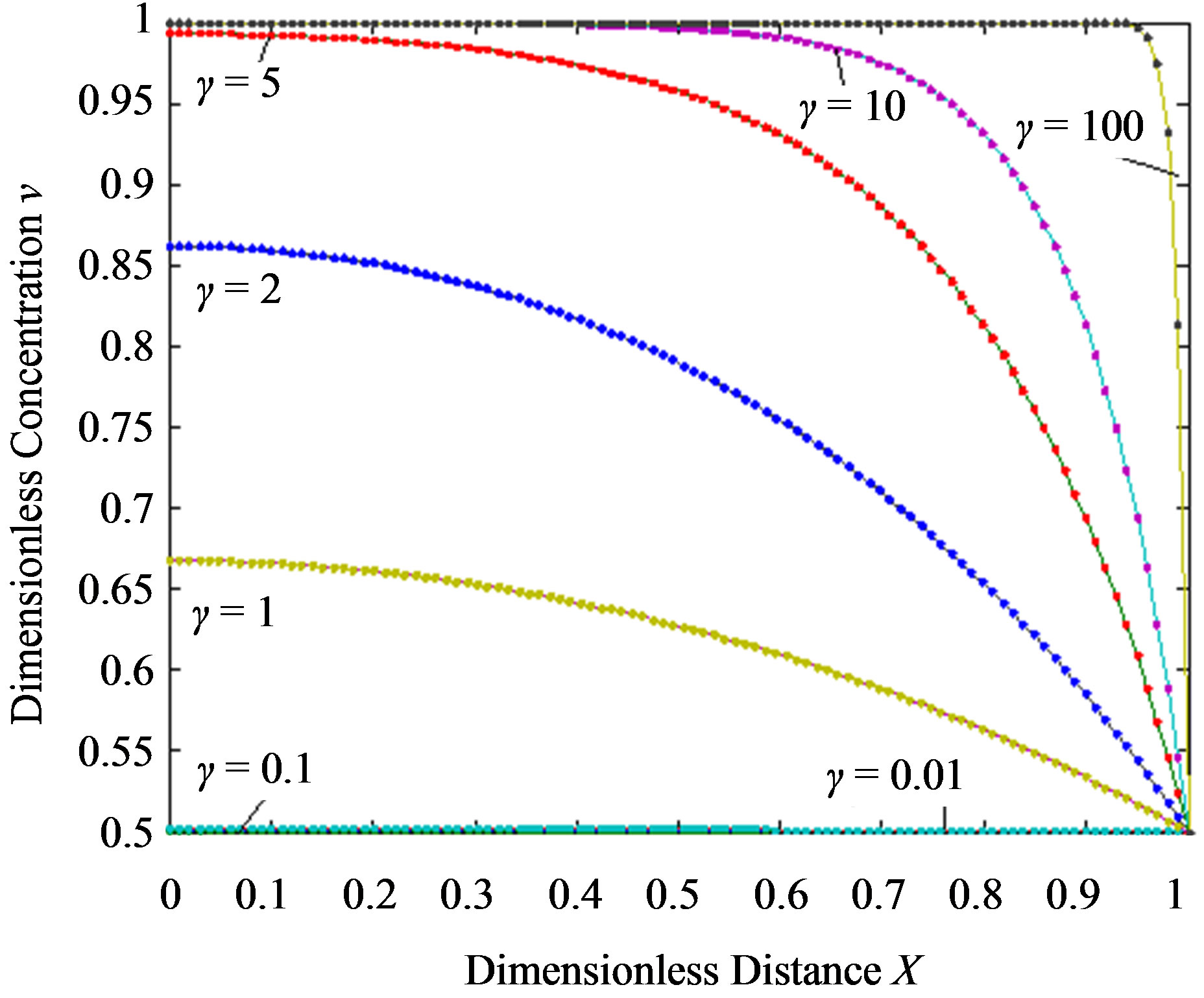 (b) α = 0.1
  (c) α = 1
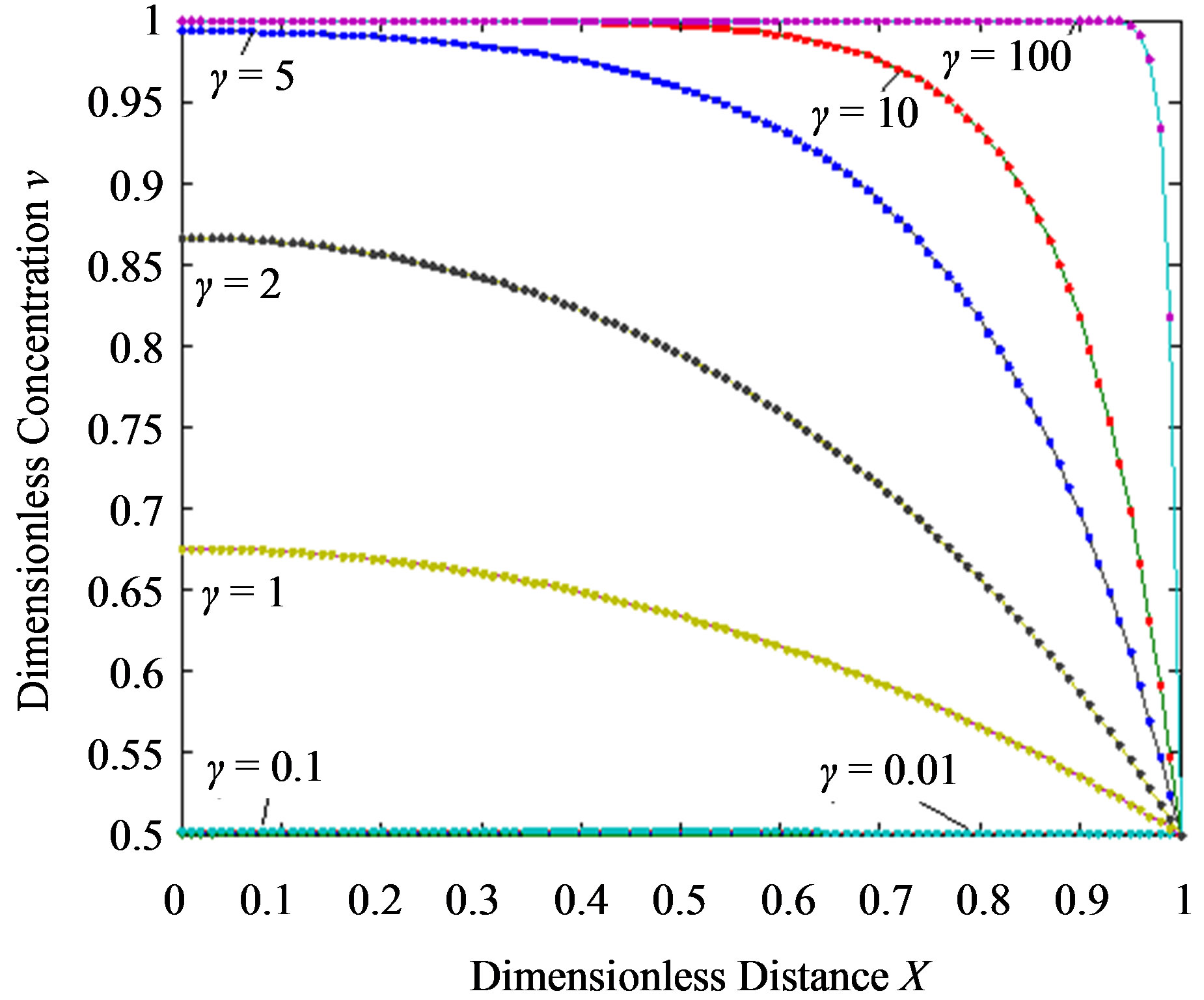
Figure 3. Dimensionless steady-state concentration profiles of the product v for various values of γ using the Eq.13. Here in all the cases , v' = 0.5 and the h value of (a), (b) is –1, and for (c) is –0.7 to –1. Solid lines represent the numerical simulation and the dotted lines represent the analytical solution.
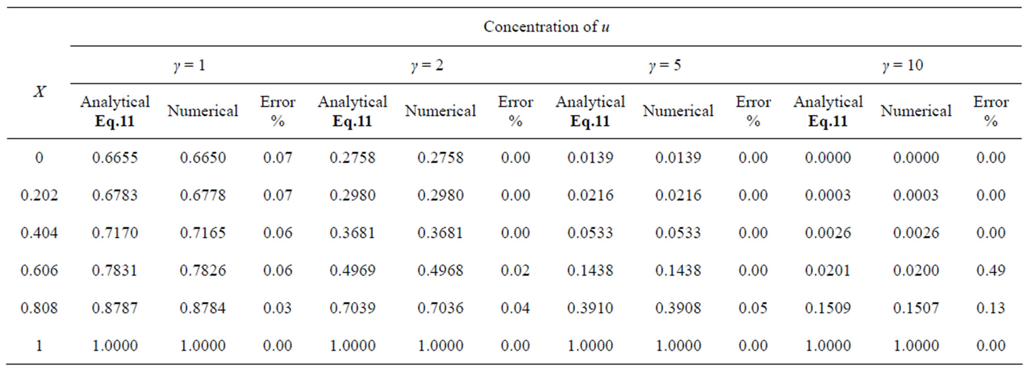
Table 1. Comparison of normalized steady-state concentration of substrate u with the numerical results for various values of γ and for some fixed values of saturation parameter α (= 0.1) and h = –1.

Table 2. Comparison of normalized steady-state concentration of substrate u vwith the numerical results for various values of γ and for some fixed values of saturation parameter α (= 1) and h = –0.5 to –0.7.
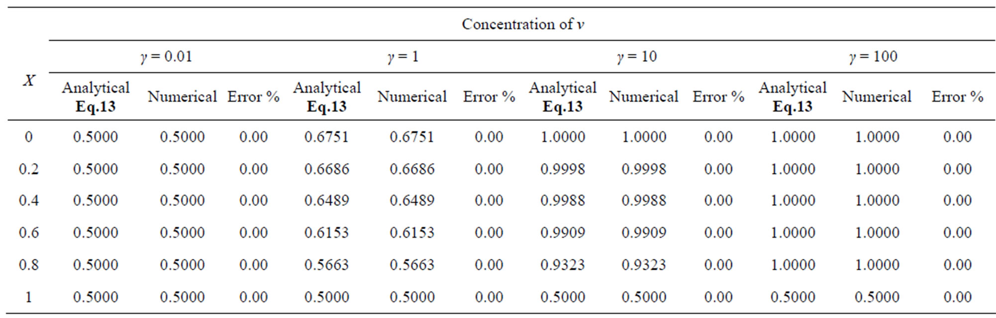
Table 3. Comparison of normalized steady-state concentration of product v th the numerical results for various values of γ and for some fixed values of saturation parameter α = 0.01, β = 0.005 and v' = 0.5. Here h = –1.

Table 4. Comparison of normalized steady-state concentration of product v with the numerical results for various values of γ and for some fixed value of saturation parameter α = 0.1, β = 0.05 and v' = 0.5. Here h = –1.
when the reaction diffusion parameter γ increases for all values of α. When γ is very small , the concentration of substrate is uniform and the curve becomes straight line. In Figures 3(a)-(c) represent the normalized concentration of product P for various values of γ.
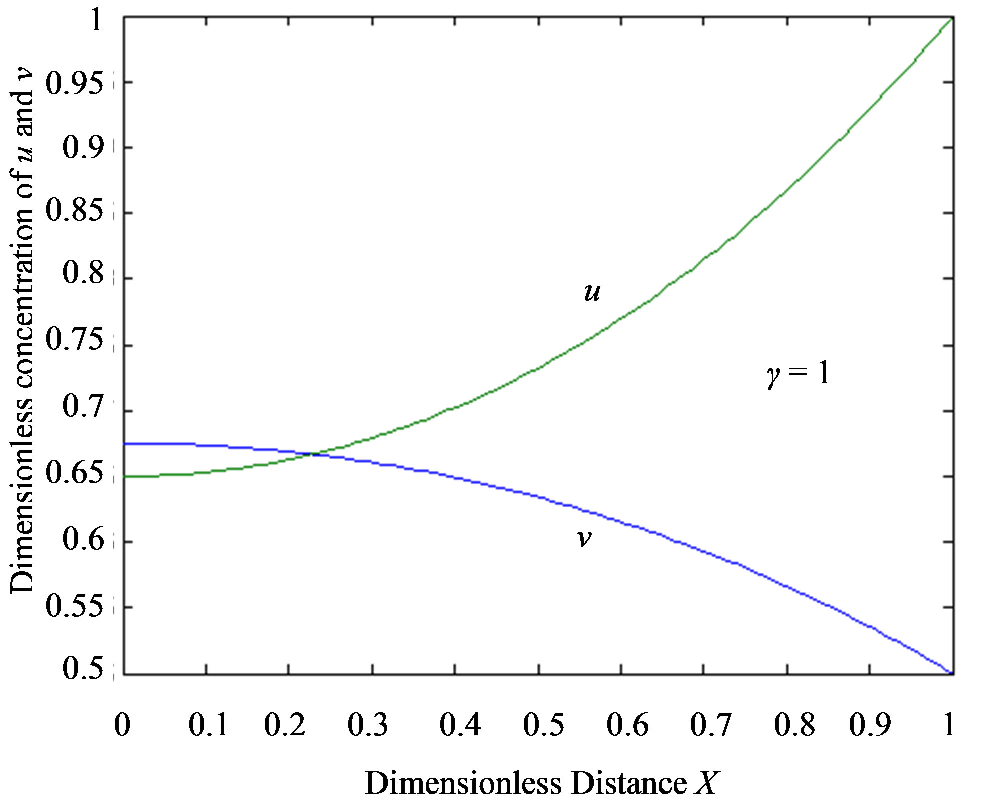
From this Figure it is obvious that the value of the product concentration P increases when the reaction diffusion parameter γ increases for various values of α. Figures 4(a) and (b) represent the normalized concentration of the substrate S and the product P for various values of γ. From this Figure it is clearly that the value of substrate concentration S decreases and the value of the product concentration P increases. From the Figures 2-4, it is also confirmed that when the thickness of the mem
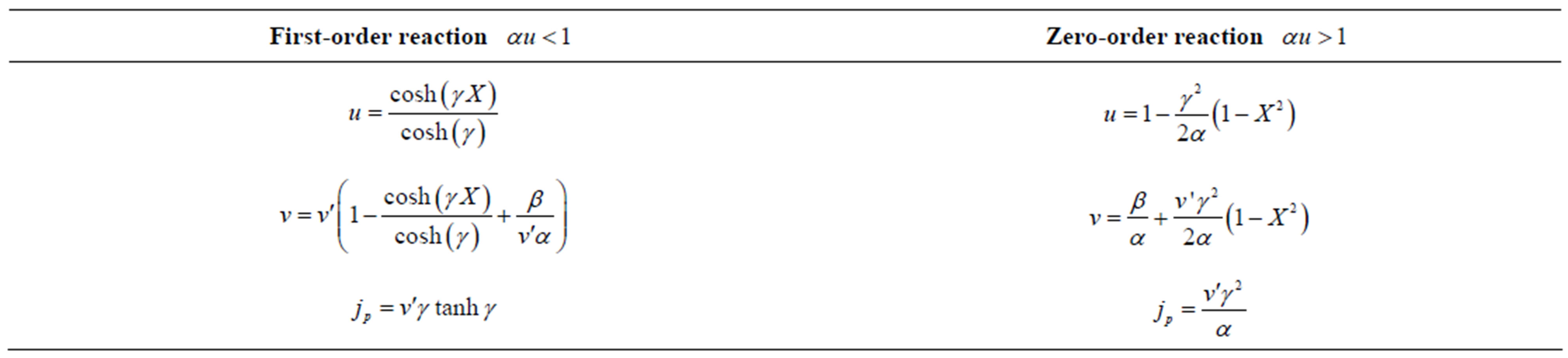
Table 5. Analytical expression of concentration of substrate, product and flux for limiting cases.
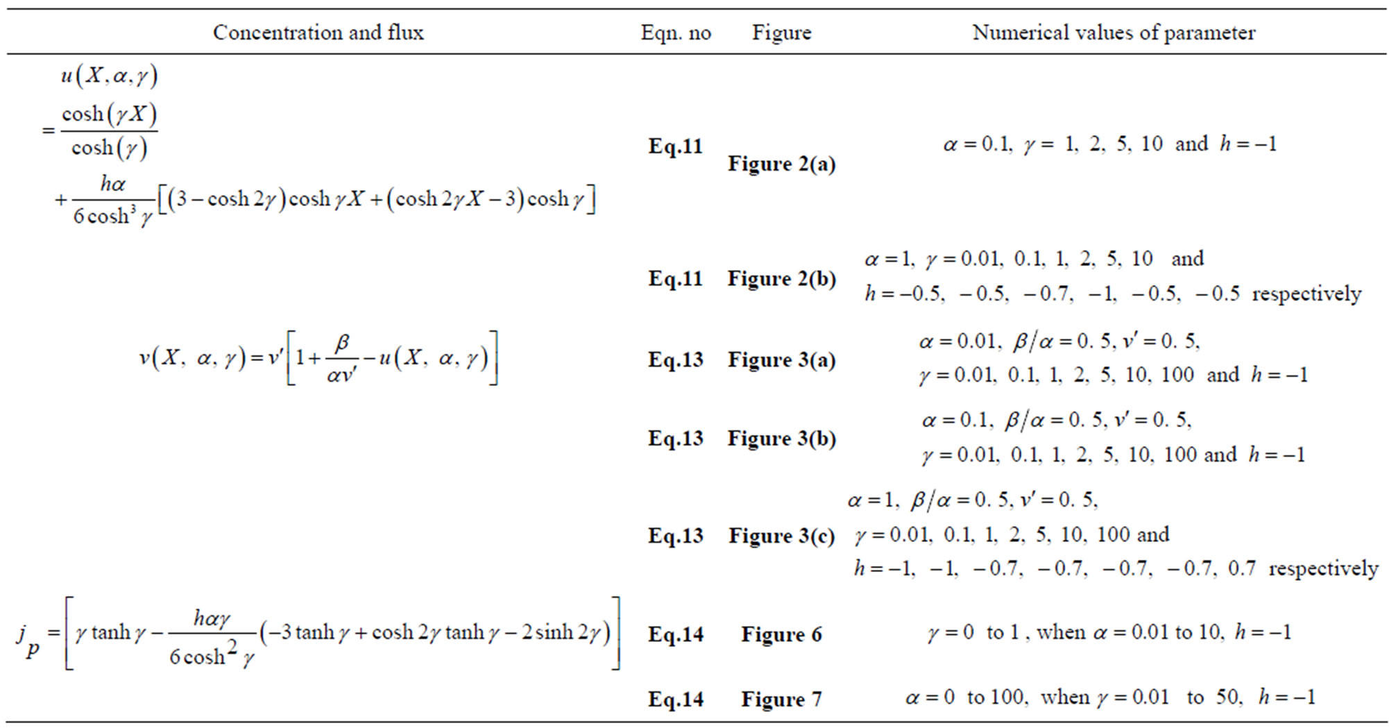
Table 6. Analytical expression of concentration of substrate, product and flux.
 (a) α = 0.01
  (b)α = 1
Figure 4.Dimensionless steady-state concentration profiles of the substrate u and product v for various values of γ using the Eqs.11, 13. Here in the above cases , v' = 0.5 and the h value of (a) and (b) is –1.
 (a)
(a)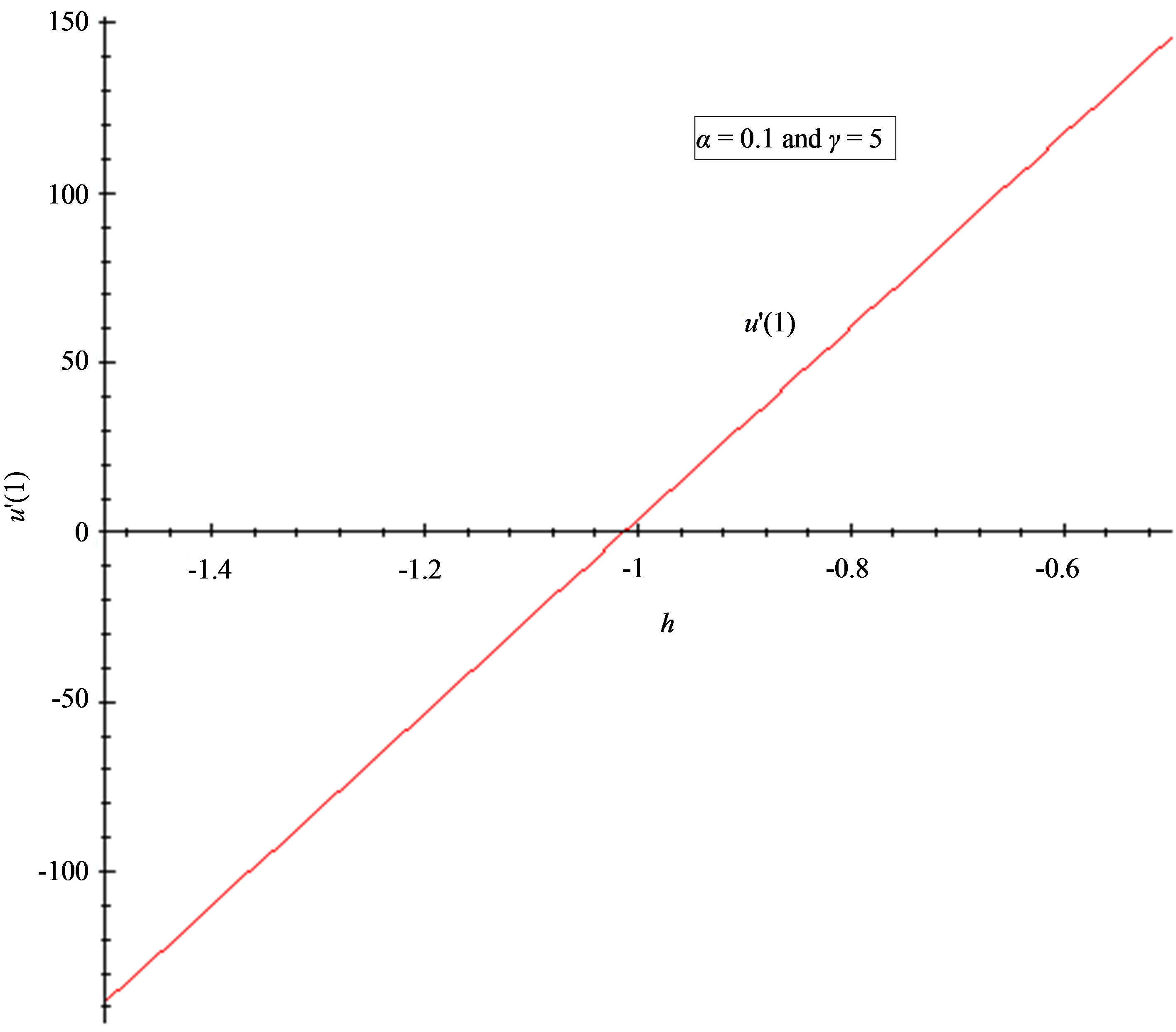 (b)
(b)
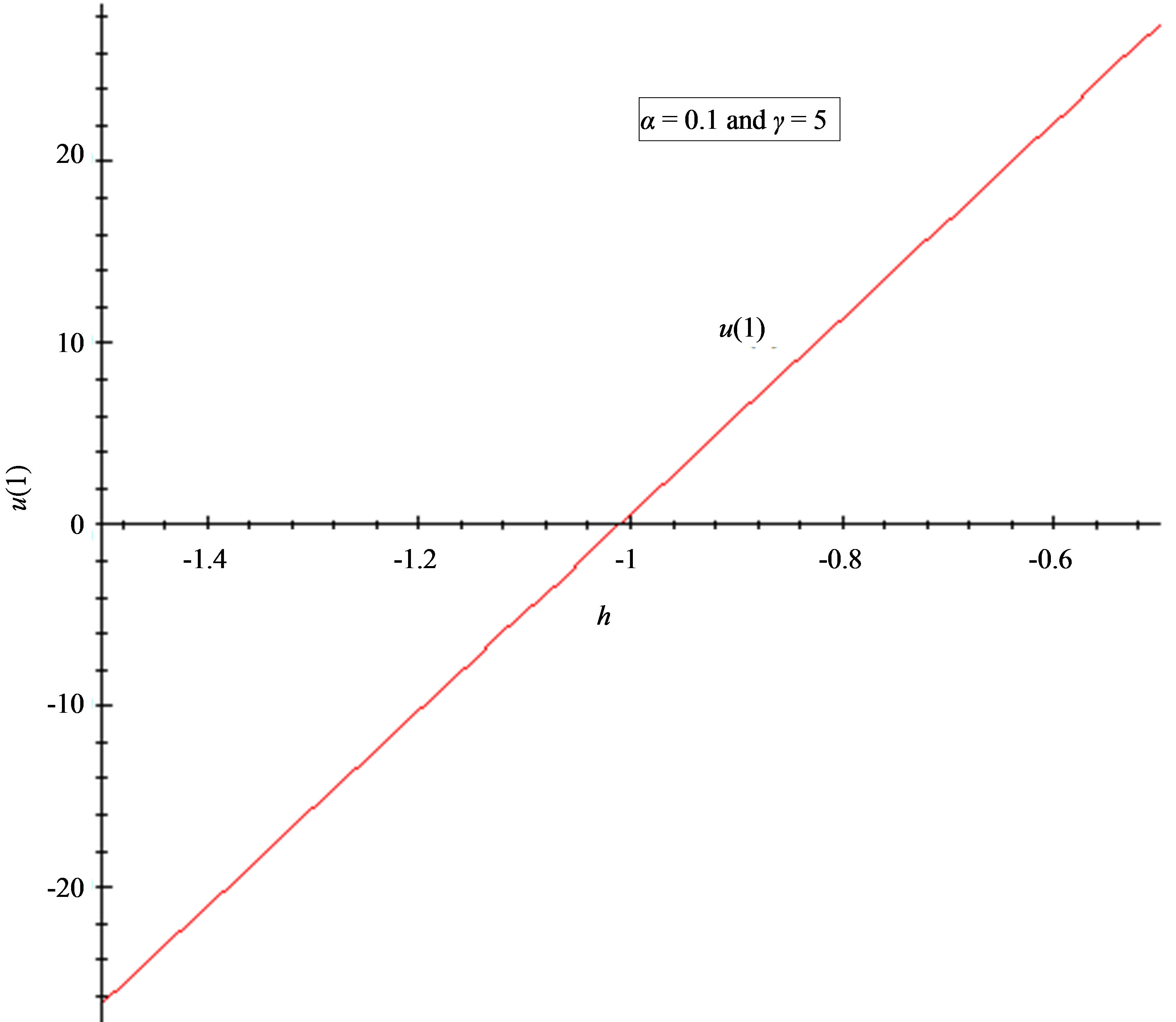
Figure 5. The h-curve of u(1) and to u'(1) given by Eq.11. (a) 2nd-order approximation of u(1); (b) 2nd-order approximation of u'(1).

Figure 6. Profiles of the dimensionless flux versus γ using the Eq.14. For α = 0.01 to 10 the value of h = –1.

Figure 7. Profiles of the dimensionless flux versus α using the Eq.14. For γ = 0.01 to 50 the value of h = –1.
brane decrease, the concentration of substrate increase and the product decrease.
7.2. Convergence Parameter h
The auxiliary convergent parameter h controls the convergence of the analytical solution series [36]. The Eq.11 and Eq.13 contain the parameter h, which gives the convergence region for the Homotophy analysis method. Multiple h curves are plotted to define the h region such that the analytical solution series is independent of h. The common region among  and its derivative
  is known as the convergence region for the corresponding function u. The h curves in Figures 5(a) and (b) represent the valid region of h is –1 when α = 0.1 and γ = 5. Similarly the value of the convergence parameter h can be obtained for different values of parameters α and γ.
7.3. Flux
The parameter of greatest interest in an amperometric biosensor is the current which is related to the flux of electroactive material to the electrode surface. For a particular membrane, the variation in γ can be achieved practically, by varying the thickness of the membrane, d, or the loading of the enzyme, . As can be seen in Eq.14, and confirmed above, the thickness appears as a squared term and thus small changes will have a much more pronounced effect on the response of the enzyme electrode than the enzyme loading.
In Figure 6 characterize the dimensionless flux versus the dimensionless reaction/diffusion parameter γ for various values of α. From this Figure, it is obvious that, the value of flux decreases when γ increases. The flux versus the dimensionless parameter α for different values of γ is plotted in Figure 7. In this Figure, the value of flux increases when γ increases. And also the current is uniform for γ ≤ 5.
8. CONCLUSION
We have theoretically analyzed the behavior of potentiometric and amperometric enzyme electrodes, which is previously described in Ref. [33]. The coupled time independent steady-state non-linear reaction/diffusion equations have been solved analytically and numerically. In this work, we have presented analytical expression corresponding to the substrate and product concentration within the polymer film in terms of parameters using Homotopy analysis method. Moreover, we have also obtained an analytical expression for the steady state current. A good agreement with numerical simulation data is noticed. The analytical results presented here will be used to determine the kinetic characteristic of the biosensor. The theoretical model described here can be used for optimization of the design of the biosensor. Further, based on the outcome of this work it is possible to extend the procedure to find the approximate amounts of substrate and product concentrations and current for reciprocal competitive inhibition process.
9. ACKNOWLEDGEMENTS
This work as supported by the Council of Scientific and Industrial Research (CSIR No.: (2442)/10/EMR-II), Government of India. (F. No. 39-58/2010(SR)), New Delhi, India. The authors are thankful to the Secretary, the Principal, The Madura College, Madurai for their encouragement.
REFERENCES
- Heller, A. and Feldman, B. (2008) Electrochemical glucose sensors and their applications in diabetes management. Chemical Reviews, 108, 2482-2505. doi:10.1021/cr068069y
- Urban, P.L., Goodall, D.M. and Bruce, N.C. (2006) Enzymatic microreactors in chemical analysis and kinetic studies. Biotechnology Advances, 24, 42-57. doi:10.1016/j.biotechadv.2005.06.001
- Blaedel, W.J., Kissel, T.R. and Boguslaski, R.C. (1972) Kinetic behavior of enzymes immobilized in artificial membranes. Analytical Chemistry, 44, 2030-2037. doi:10.1021/ac60320a021
- Guilbault, G.G. and Nagy, G.G. (1973) Improved urea electrode. Analytical Chemistry, 45, 417-419. doi:10.1021/ac60324a053
- Hameka, H.F. and Rechnitz, G.A. (1983) Theory of the biocatalytic membrane electrode. Journal of Physical Chemistry, 87, 1235-1241. doi:10.1021/j100230a029
- Tranh-Minh, C. and Broun, G. (1975) Construction and study of electrodes using cross-linked enzymes. Analytical Chemistry, 47, 1359-1364. doi:10.1021/ac60358a075
- Morf, W.E. (1980) Theoretical evaluation of the performance of enzyme electrodes and of enzyme reactors. Microchimica Acta, 74, 317-332. doi:10.1007/BF01196457
- Morf, W.E. (1981) The principles of ion-selective electrodes and of membrane transport. Elsevier, New York.
- Glab, S., Koncki, R. and Hulanicki, A. (1991) Kinetic model of pH-based potentiometric enzymic sensors. Part 1. Theoretical considerations. Analyst (London), 116, 453- 480. doi:10.1039/an9911600453
- Glab, S., Koncki, R. and Holona, I. (1992) Kinetic model of pH-based potentiometric enzymic sensors. Part 2. Method of fitting. Analyst (London), 117, 1671-1674. doi:10.1039/an9921701671
- Glab, S., Koncki, R. and Hulanicki, A. (1992) Kinetic model of pH-based potentiometric enzymic sensors. Part 3. Experimental verifications. Analyst (London), 117, 1675- 1678. doi:10.1039/an9921701675
- Mell, L.D. and Maloy, J.T. (1975) A model for the amperometric enzyme electrode obtained through digital simulation and applied to the immobilized glucose oxidase system. Analytical Chemistry, 47, 299-307. doi:10.1021/ac60352a006
- Mell, L.D. and Maloy, J.T. (1976) Amperometric response enhancement of the immobilized glucose oxidase enzyme electrode. Analytical Chemistry, 48, 1597-1601. doi:10.1021/ac50005a045
- Olsson, B., Lundback, H. and Johansson, G. (1986) Theory and application of diffusion-limited amperometric enzyme electrode detection in flow injection analysis of glucose. Analytical Chemistry, 58, 1046-1052. doi:10.1021/ac00297a014
- Albery, W.J. and Bartlett, P.N. (1985) Amperometric enzyme electrodes. Journal of Electroanalytical Chemistry, 194, 211-222. doi:10.1016/0022-0728(85)85005-1
- Albery, W.J., Bartlett, P.N., Driscoll, B.J. and Lennox, R.B. (1992) Amperometric enzyme electrodes. 5. The homogeneous mediated mechanism. Journal of Electroanalytical Chemistry, 323, 77-102. doi:10.1016/0022-0728(92)80004-N
- Mackey, D., Killard, A.J., Ambrosi, A. and Smyth, M.R. (2007) Optimizing the ratio of horseradish peroxidase and glucose oxidase on a bienzyme electrode: Comparison of a theoretical and experimental approach. Sensors & Actuators B, 122, 395-402. doi:10.1016/j.snb.2006.06.006
- Matsue, T., Yamada, H., Chang, H.C., Uchida, I., Nagata, K. and Tomita, K. (1990) Electron transferase activity of diaphorase (NADH: acceptor oxidoreductase) from Bacillus stearothermophilus. Biochimica et Biophysica Acta, 1038, 29-38. doi:10.1016/0167-4838(90)90006-2
- Yokoyama, K. and Kayanuma, Y. (1998) Cyclic voltammetric simulation for electrochemically mediated enzyme reaction and determination of enzyme kinetic constants. Analytical Chemistry, 70, 3368-3376.
- Baronas, R., Kulys, J. and Ivanauskas, F. (2004) Modelling amperometric enzyme electrode with substrate cyclic conversion. Biosensors & Bioelectronics, 19, 915-922. doi:10.1016/j.bios.2003.08.022
- Morf, W.E., Pretsch, E. and de Rooij, N.F. (2007) Computer simulation of ion-selective membrane electrodes and related systems by finite-difference procedutres. Journal of Electroanalytical Chemistry, 602, 43-54. doi:10.1016/j.jelechem.2006.11.025
- Morf, W.E., Pretsch, E. and de Rooij, N.F. (2008) Theory and computer simulation of the time-dependent selectiveity behavior of polymeric membrane ion-selective electrodes. Journal of Electroanalytical Chemistry, 614, 15- 23. doi:10.1016/j.jelechem.2007.10.027
- Morf, W.E., Pretsch, E. and de Rooij, N.F. (2009) Memory effects of ion-selective electrodes: Theory and computer simulation of the time-dependent potential response to multiple sample changes. Journal of Electroanalytical Chemistry, 633, 137-145. doi:10.1016/j.jelechem.2009.05.004
- Morf, W.E., Pretsch, E. and de Rooij, N.F. (2010) Theoretical treatment and numerical simulation of potential and concentration profiles in extremely thin non-electroneutral membranes used for ion-selective electrodes. Journal of Electroanalytical Chemistry, 641, 45-56. doi:10.1016/j.jelechem.2010.01.001
- Sandifer, J.R. and Buck, R.P. (1975) Algorithm for simulation of transient and alternating current electrical properties of conducting membranes, junctions, and one-dimensional, finite galvanic cells. Journal of Physical Chemistry, 79, 384-391. doi:10.1021/j100571a019
- Brumleve, T.R. and Buck, R.P. (1978) Numerical-solution of nernst-planck and poisson equation system with applications to membrane electrochemistry and solid-state physics. Journal of Electroanalytical Chemistry, 90, 1-31. doi:10.1016/S0022-0728(78)80137-5
- Sokalski, T. and Lewenstam, A. (2001) Application of nernst-plank equation and poisson equations for interpretation of liquid junction and membran potential in real-time and space domains. Electrochemistry Communications, 3, 107-112. doi:10.1016/S1388-2481(01)00110-2
- Sokalski, T., Lingenfelter, P. and Lewenstam, A. (2003) Numerical solution of the coupled Nernst-Planck and Poisson equations for liquid-junction and ion-selective membrane potentials. Journal of Physical Chemistry B, 117, 2443-2452. doi:10.1021/jp026406a
- Lingenfelter, P., Bedlechowicz-Silwachowska, I., Sokalski, T., Maj-Zurawska, M. and Lewenstam, A. (2006) Time-dependent phenomena in the potential response of ion-selective electrodes treated by the nernst-planckpoisson model. 1. Intramembrane processes and selectivity. Analytical Chemistry, 78, 6783-6791. doi:10.1021/ac060264p
- Bobacka, J., Ivaska, A. and Lewenstam, A. (2008) Potentiometric ion sensors. Chemical Reviews, 108, 329-351. doi:10.1021/cr068100w
- Stryer, L. (1975) Biochemistry. Freeman, San Francisco.
- Reithel, F.J. (1971) Ureases. In: Boyer, P.D. Ed., The Enzymes, 3rd Edition, Academic Press, New York.
- Morf, W.E., van der Wal, P.D., Pretsch, E. and de Rooji, N.F. (2011) Theoretical treatment and numerical simulation of potentiometric and amperometric enzyme electrodes and of enzyme reactors. Part 2: Time-dependent concentration profiles, fluxes, and responses. Journal of Electroanalytical Chemistry, 657, 1-12. doi:10.1016/j.jelechem.2011.02.007
- Morf, W.E., van der Wal, P.D., Pretsch, E. and de Rooji, N.F. (2011) Theoretical treatment and numerical simulation of potentiometric and amperometric enzyme electrodes and of enzyme reactors. Part 1: Steady-state concentration profiles, fluxes, and responses. Journal of Electroanalytical Chemistry, 657, 13-22. doi:10.1016/j.jelechem.2011.02.006
- Liao, S.J. (2012) The homotopy analysis method in nonlinear differential equations. Springer and Higher Education press, New York. doi:10.1007/978-3-642-25132-0
- Liao, S.J. (2003) Beyond perturbation: An introduction to the homotopy analysis method. Chapman & Hall/CRC Press, Boca Raton. doi:10.1201/9780203491164
- Allan, F.M. (2007) Derivation of the adomian decomposition method using the homotopy analysis method. Applied Mathematics and Computation, 190, 6-14. doi:10.1016/j.amc.2006.12.074
- Liao, S.J. (2003) The proposed homotopy analysis technique for the solution of nonlinear problems. Ph.D. Thesis, Shanghai Jiao Tong University, Shanghai.
- Liao, S.J. (2004) On the homotopy analysis method for nonlinear problems. Applied Mathematics and Computation, 147, 499-513. doi:10.1016/S0096-3003(02)00790-7
- Loghambal, S. and Rajendran, L. (2011) Analytical expressions of concentration of nitrate pertaining to the electrocatalytic reduction of nitrate ion. Journal of Electroanalytical Chemistry, 661, 137-143. doi:10.1016/j.jelechem.2011.07.027
- Liao, S.J. (2009) The proposed homotopy analysis tecnique for the solution of nonlinear problems. Communications in Nonlinear Science and Numerical Simulation, 14, 983-997. doi:10.1016/j.cnsns.2008.04.013
- Liao, S.J. and Tan, Y. (2007) A general approach to obtain series solutions of nonlinear differential equations. Studies in Applied Mathematics, 119, 297-355. doi:10.1111/j.1467-9590.2007.00387.x
- Liao, S.J. (2003) Beyond perturbation: Introduction to the homotopy analysis method. Chapman and Hall, CRC Press, Boca Raton, 336.
- Domairry, G. and Fazeli, M. (2009) Homotopy analysis method to determine the fin efficiency of convective straight fins with temperature-dependent thermal conductivity. Communications in Nonlinear Science and Numerical Simulation, 14, 489-499. doi:10.1016/j.cnsns.2007.09.007
APPENDIX A: ANALYTICAL SOLUTION OF EQ.7 USING HOMOTOPY ANALYSIS METHOD
The zero-order deformation equation of non-linear Eq.7 is
 (A1)
(A1)
where  is an embedding parameter and
  is the so-called convergence parameter. When p = 0, the Eq.A1 becomes
 (A2)
(A2)
The boundary conditions are
 . (A3)
The solution of Eq.A2 using boundary condition (A3) is
 . (A4)
When  the Eq.A1 is equivalent to Eq.7. Thus it holds
 . (A5)
Expanding  in Taylor series with respect to the embedding parameter p, we have,
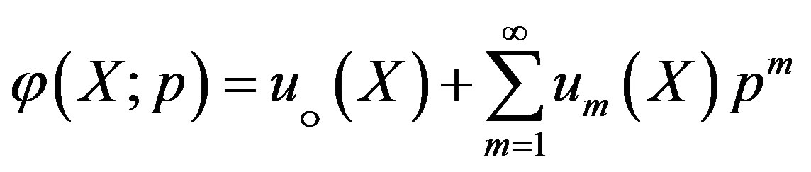 (A6)
(A6)
where
 (A7)
(A7)
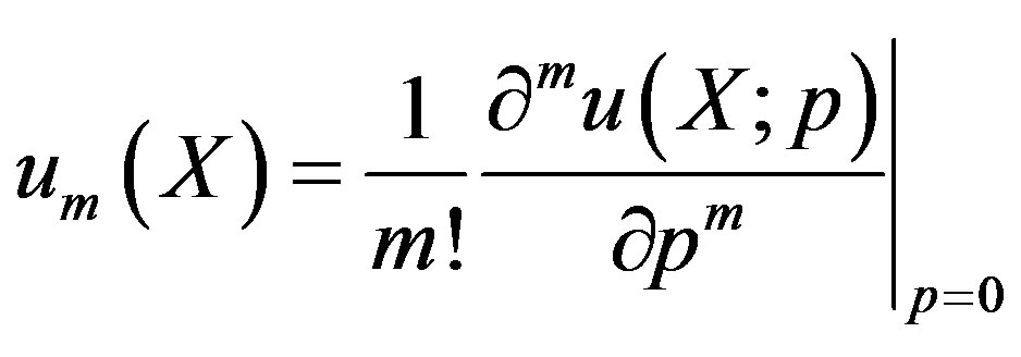 (A8)
(A8)
Note that the series Eq.A6 contains the convergence control parameter h. Assuming that h is chosen so properly that the above series is convergent at . We have the solution series as
 (A9)
(A9)
Substituting Eq.A6 into the zeroth-order deformation Eq.A1 and equating the co-efficient of p we have,
 (A10)
(A10)
The boundary conditions are
 (A11)
(A11)
From Eq.A10 we get
 (A12)
(A12)
Adding Eqs.A4 and A12, we get Eq.11 in the text.
APPENDIX B: MATLAB/SCILAB PROGRAM TO FIND THE NUMERICAL SOLUTION OF THE EQS.7 AND 8
function pdex4 m = 0;
x = linspace(0,1); %d=1 t=linspace(0,10);
sol = pdepe(m,@pdex4pde,@pdex4ic,@pdex4bc,x,t);
u1 = sol(:,:,1);
u2 = sol(:,:,2);
figure plot(x,u1(end,:))
title('u1(x,t)')
xlabel('Distance x')
ylabel('u1(x,2)')
%-----------------------------------------------------------------
figure plot(x,u2(end,:))
title('u2(x,t)')
xlabel('Distance x')
ylabel('u2(x,2)')
% -------------------------------------------------------------
function [c,f,s] = pdex4pde(x,t,u,DuDx)
c = [1; 1];
f = [1; 1] .* DuDx;
gamma=100;
alpha=100;
v=0.1;
%beta=0.5;
F=-(gamma^2*u(1))/(alpha*u(1)+1);
F1=(v*(gamma^2*u(1)/(alpha*u(1)+1)));
s=[F; F1];
% -------------------------------------------------------------
Functionu0=pdex4ic(x); %create a initial conditions u0 = [1; 1];
% -------------------------------------------------------------
function[pl,ql,pr,qr]=pdex4bc(xl,ul,xr,ur,t)
%create a boundary conditions pl = [0; 0];
ql = [1; 1];
pr = [ur(1)-1; ur(2)];
qr = [0; 0];
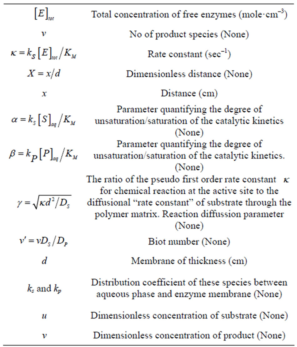
APPENDIX C: NOMENCLATURE AND UNITS