ABSTRACT

The question of the averaging of inhomogeneous spacetimes in cosmology is important for the correct interpretation of cosmological data. In this paper a conceptually simpler approach to averaging in cosmology is suggested, based on the averaging of scalars within unimodular gravity. As an illustration, the example of an exact spherically symmetric dust model is considered, and it is shown that within this approach averaging introduces correlations (corrections) to the effective dynamical evolution equation in the form of a spatial curvature term.

1. Introduction

The Universe is not isotropic or spatially homogeneous on local scales. The correct governing equations on cosmological scales are obtained by averaging the gravitational field equations (FE). An averaging of inhomogeneous spacetimes in Einstein’s general relativity (GR) can lead to dynamical behavior different from the spatially homogeneous and isotropic Friedmann-LemaîtreRobertson-Walker (FLRW) model; in particular, the expansion rate may be significantly affected [1-3]. Consequently, a solution of the averaging problem is of considerable importance for the correct interpretation of cosmological data.

The solution to this problem necessitates a method for covariantly (and gauge invariantly) averaging tensors on a background differential manifold. Unfortunately, this is a very difficult problem. In the Isaacson spacetime averaging scheme in macroscopic gravity (MG) bilocal averaging operators are utilized [4-8]. Choosing a compact region in an (n-dimensional differentiable) manifold (,) with a volume -form and a supporting point to which the average value will be prescribed, the average value of a geometric object, , over a region (with volume) at, is defined in terms of the bilocal extension of the object, , by means of the bilocal averaging operator. The averaging scheme is covariant and linear by construction, and the averaged object has the same tensorial character as. In any manifold with a volume -form there always exist locally volume-preserving divergence-free operators [6-8], in which the bilocal operator takes the simplest possible form: [9].

The definition of an average consequently takes on a particularly simple form when written in a volume-preserving (system of) coordinates (VPC). Indeed, if the manifold is a pseudo-Riemannian spacetime, the spacetime average of a tensor field, at a supporting point in VPC is thus

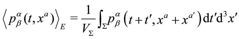(1)

In the MG covariant approach to the averaging problem the Einstein FE (EFE) on cosmological scales with a continuous distribution of cosmological matter are modified by appropriate gravitational correlation (correction) terms [4,6-8]. The averaged FE can always be written in the form of the FE for the macroscopic metric tensor when the correlation terms are moved to the right-hand side of the averaged field equations, and consequently can be regarded as a geometric modification to the averaged (macroscopic) matter energy-momentum tensor [4,6-8]. In [10] it was found that by solving the MG equations the averaged EFE for a spatially homogeneous, isotropic macroscopic spacetime geometry has the form of the EFE of GR for an FLRW geometry with an additional spatial curvature term (i.e., the correlation tensor is of the form of a spatial curvature term) (see also [11,12]). Unfortunately, the spacetime averaging scheme in MG is very difficult to apply and is fraught with complications [13]. In this paper an alternative approach to averaging is suggested, exploiting the preferred nature of VPC and based on the averaging of scalars [14-16].

2. Unimodular Gravity

The fundamental variables in the action for unimodular gravity and the Einstein-Hilbert action for GR are different [17-20]. In unimodular gravity, there is an additional restriction on the metric, not present in GR: the determinant of g_uv equals one. As a consequence of, unimodular gravity is only invariant under volume-preserving diffeomorphisms.¹ Thus, unimodular gravity presents a natural theory in which to do averaging.

Varying the action in unimodular gravity leads to the FE relating the traceless Ricci tensor, 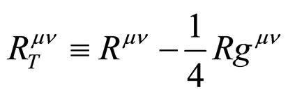to the corresponding traceless energy-momentum tensor [17]. It should be noted that the energy-momentum conservation law does not follow from this equation of motion, but has to be imposed separately. Assuming energy-momentum conservation, it then follows that

(2)

where is a constant (and and). Using the contracted Bianchi identity, , we then obtain

where is given in terms of and the vacuum energy density (part of the energy-momentum tensor). Hence the cosmological constant naturally appears in terms of a constant of integration in unimodular gravity.

Therefore, the theory acquires a new integrability condition [17]. Both the trace-free FE and the matter conservation equations are assumed; the integrability condition follows from these equations. Hence, we obtain the differential relations which are functionally equivalent to the full EFE (where the spacetime volume density is not a dynamical variable), where the cosmological constant is thus given in terms of an arbitrary integration constant and is not given explicitly by the vacuum energy.

This is an old proposal essentially initiated by Einstein [21-23] and more recently it has been developed under the name of unimodular gravity [18-20,24]. It has been suggested that unimodular gravity can be used to eliminate problems caused by the nature of the cosmological constant as well as to resolve the discrepancies between theory and observation, while not introducing any exotic terms such as quintessence or dark energy into the analysis of the EFE [18-20,25]. Indeed, although unimodular gravity does not give a unique value for the effective cosmological constant, it has the potential to solve the huge discrepancy between theory and observation. With a suitable high-energy cut-off, the vacuum energy density is estimated by Weinberg [17] to be of the order, whereas the effective value of the cosmological constant as determined by astronomical observations is of the order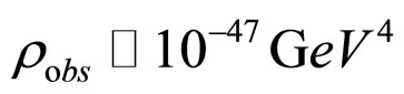. However, there is no longer a cosmological constant problem. For example, for a perfect fluid the matter source term is the manifestly trace-free stress tensor; hence, matter enters the FE only in terms of the inertial mass density, which vanishes in the case of a cosmological constant (e.g., see [26,27]).

Unimodular gravity has also been utilized in the study of the quantization of GR [20,24]. The Hamiltonian of a generally covariant theory is zero, so in a sense there is no evolution, but since unimodular gravity is not generally covariant, the classical  problem of time is avoided [20]. In addition, in unimodular gravity quantum gravitational factor ordering ambiguities are alleviated [24].

3. Averaging Proposal

We wish to exploit the structure of unimodular gravity to suggest an alternative approach to averaging in cosmology. Within unimodular gravity we need to average the trace-free part of the FE and the trace of the FE separately.

1) Average trace-free part of the FE: Here the resulting correlation tensor must consequently be trace-free. If the form of the resulting equations are of the algebraic form of a “perfect fluid”, as in the cosmological application (with a large scale FLRW geometry), then the correlation tensor must be of the form of an effective energy momentum tensor for which the trace, corresponding to a radiation fluid [28]. Note that if the matter is dust, then

which could be (trivially) reinterpreted as a renormalized dust term (with energy density) and a term corresponding to a constant spatial curvature (with) [10-12].

2) Average trace of the FE: In this case we only need to work with the (generalized) Friedmann Equation (2).²

The problem of averaging is then effectively reduced to considering the average of a single scalar eqn (see [14]).

4. Example: Lematre-Tolman-Bondi Model

The exact spherically symmetric dust Lematre-TolmanBondi (LTB) model [30], which can be regarded as an exact inhomogeneous generalization of the FLRW solution, can be rewritten in VPC [11,12]. Taking, the line-element becomes

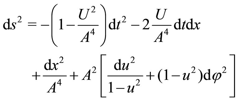(3)

which has 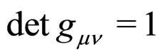as desired, where is defined as

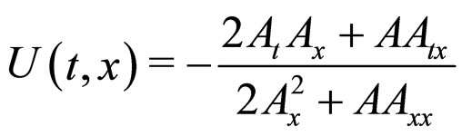(4)

The constraints on the original LTB metric ensuring a dust solution are given in [11,12]. For general functions and, the Ricci scalar of the metric (3) is given by

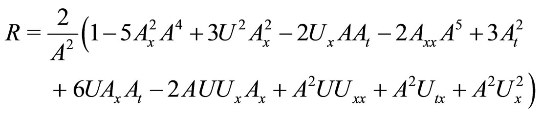(5)

The spatially flat () FLRW model in VPC is given by the metric (3) with

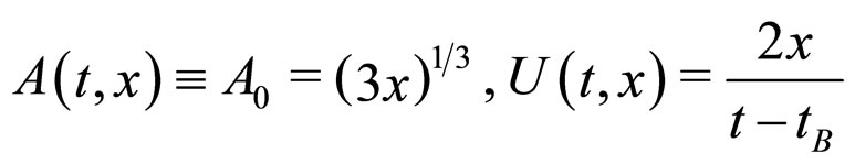(6)

where, strictly speaking, the degenerate form for U(t,x) does not follow directly from Equation (4) (however, Equation (5) is valid for (6) and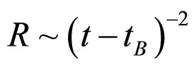). Defining, the Ricci scalar of the FLRW metric with positive curvature constant is given by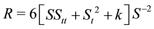. For the zero-curvature Einstein de-Sitter metric, , and setting, we get the approximate expression:

(7)

consistent with the expression given in [11,12] (with ).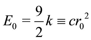

A Perturbative Solution

Let us assume that is zero, which implies that the bang time is uniform and we are consequently restricting our choice of LTB models to those with no decaying modes. We shall also consider solutions of the LTB metric in VPC as perturbations about the spatially flat FLRW model given by (6). In this respect our approximate solution will be an expansion with respect to and we require the Einstein tensor to have the form of dust (after truncation of terms of or higher). We begin by making the formal expansion for in the form:

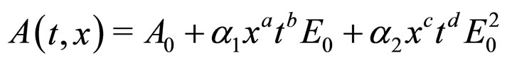(8)

where, , a, b, c and d are constants. We can use Equations (4) and (8) to obtain. Calculating the Einstein tensor and requiring it have the form of dust (up to order) allows us to determine the constants in our perturbative solution (we obtain:, , and [11,12]).

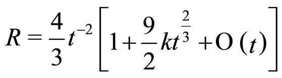
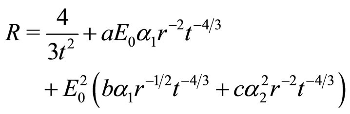
The expression that results from substituting in terms of A using Equation (4) and the expression (8) for A (with the given powers of and in our particular perturbative solution) leads to the expression for the Ricci scalar (keeping only terms up to):

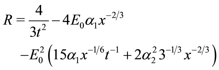(9)

Defining, we obtain

(10)

where

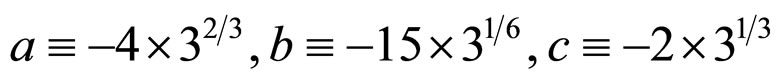(11)

Finally, we obtain the averaged version of the Ricci scalar equation by integrating Equation (10) over the radial variable, where is the (radial) averaging length scale:

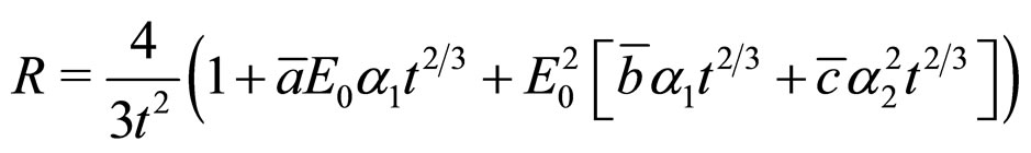(12)

(where the “barred” constants are the appropriately - renormalized constants). We see that all of the correction terms (correlations) introduced by averaging the Ricci scalar equation are of the form of a spatial curvature term (7), which is consistent with the results of [11,12].³

5. Discussion

Recent observations are usually interpreted as implying that the Universe is very nearly flat, currently accelerating and indicating the existence of dark matter and dark energy [31-33]. A cosmological constant is a candidate for the dark energy. Averaging can have a very significant dynamical effect on the evolution of the Universe; the correction terms change the interpretation of observations so that they need to be accounted for carefully to determine if the models may be consistent with an accelerating Universe. Indeed, it has been argued that a more conservative approach to explain the acceleration of the Universe without the introduction of exotic fields might be to utilize a backreaction effect due to inhomogeneities of the Universe.

In this paper we have argued that a rigorous approach to cosmological averaging (and necessary for studying cosmological data) is perhaps most naturally studied within the context of unimodular gravity. In the simple example studied here, we found that all correction terms introduce correlations of the form of a spatial curvature term [11,12].

As another simple illustration, we can consider the special case () of the exact solution representing a two-scale Buchert average of the EFE for an inhomogeneous universe approximating the observed Universe [34]. This exact solution has voids surrounded by walls (within which clusters of galaxies are located). The geometry within a wall is given by 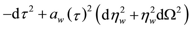and the geometry within a void has negative curvature.

The averaging procedure leads to the equations

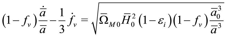
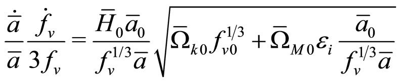
where is an integration constant, and are the matter and curvature parameters, respectively, and and are the volume fractions occupied by voids and walls. For the averaged cosmic scale factorwe find that

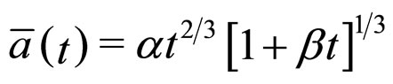
where

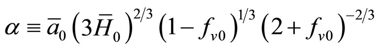
and

.

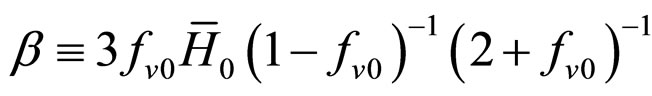In this example, the Ricci scalar is again of the form of Equation (7).

In future work we intend to consider this averaging scheme in more general cosmological contexts. In particular, we wish to study approximate solutions within linear perturbation theory. A first step will be to develop perturbation theory within unimodular gravity [35,36].

6. Acknowledgements

This work was supported, in part, by NSERC.

REFERENCES

NOTES

^*Current address: Department of Mathematics, Physics and Geology, Cape Breton University, Sydney, Canada.

¹Coordinate invariance can always be reinstated into the theory.

²Note that the sum of the averaged energy-momentum tensor and the correlation tensor is covariantly conserved; the question of whether the averaged energy-momentum is separately conserved with respect to the averaged geometry is determined by averaging the energy-momentum conservation equation (if it is not, then there is an effective interation between the averaged energy-momentum tensor and the correlation tensor [29]).

³We note that for this perturbative solution, we obtain higher order correction terms of the form, which can be interpreted as a renormalization of in the exact dust solution. We also note that, in principle, for the second order terms () to be formally comparable,.

REFERENCES

- G. F. R. Ellis, “Gelativistivc Cosmology: Its Nature Aims and Problems,” In: B. Bertotti, F. de Felici and A. Pascolini, Eds., General Relativity and Gravitation, Reidel, Dordrecht, 1984, pp. 215-588.
- G. F. R. Ellis and W. Stoeger, “Perturbed Spherically Symmetric Dust Solution of the Field Equations in Observational Coordinates with Cosmological Data Functions,” Classical Quantum Gravity, Vol. 4, No. 6, 1987, p. 1697. doi:10.1088/0264-9381/4/6/025
- G. F. R. Ellis and T. Buchert, “The Universe Seen at Different Scales,” Physics Letters A, Vol. 347, No. 1-3, 2005, pp. 38-46. doi:10.1016/j.physleta.2005.06.087
- R. A. Isaacson, “Gravitational Radiation in the Limit of High Frequency. I. The Linear Approximation and Geometrical Optics,” Physical Reviews, Vol. 166, No. 5, 1968, pp. 1263-1272. doi:10.1103/PhysRev.166.1263
- R. A. Isaacson, “Gravitational Radiation in the Limit of High Frequency. II. Nonlinear Terms and the Effective Stress Tensor,” Physical Reviews, Vol. 166, No. 5, 1968, pp. 1272-1280. doi:10.1103/PhysRev.166.1272
- R. M. Zalaletdinov, “Averaging Problem in Cosmology and Macroscopic Gravity,” General Relativity Gravitation, Vol. 24, No. 10, 1992, pp. 1015-1031. doi:10.1007/BF00756944
- R. M. Zalaletdinov, “Towards a Theory of Macroscopic Gravity,” General Relativity Gravitation, Vol. 25, No. 7, 1993, pp. 673-695. doi:10.1007/BF00756937
- R. M. Zalaletdinov, “The Gravitational Polarization in General Relativity: Solution to Szekeres’ Model of Quadrupole Polarization,” General Relativity Gravitation, Vol. 20, No. 19, 2003, pp. 4195-4212.
- M. Mars and R. M. Zalaletdinov, “Space-Time Averages in Macroscopic Gravity and Volume-Preserving Coordinates,” Journal of Mathematical Physics, Vol. 38, No. 9, 1997, p. 4741. doi:10.1063/1.532119
- A. A. Coley, N. Pelavas and R. M. Zalaletdinov, “Cosmological Solutions in Macroscopic Gravity,” Physical Review Letters, Vol. 95, No. 15, 2005, p. 151102. doi:10.1103/PhysRevLett.95.151102
- A. A. Coley and N. Pelavas, “Averaging in Spherically Symmetric Cosmology,” Physical Review D, Vol. 75, No. 4, 2006, p. 043506. doi:10.1103/PhysRevD.75.043506
- A. A. Coley and N. Pelavas, “Averaging in Spherically Symmetric Cosmology,” Physical Review D, Vol. 74, No. 8, 2006, p. 087301. doi:10.1103/PhysRevD.74.087301
- J. Brannlund, R. J. van den Hoogen and A. Coley, “Averaging Geometrical Objects on a Differentiable Manifold,” International Journal of Modern Physics D, Vol. 19, No. 12, 2010, pp. 1915-1923. doi:10.1142/S0218271810018062
- A. Coley, “Averaging in Cosmological Models Using Scalars,” Classical Quantum Gravity, Vol. 27, No. 24, 2010, p. 245017. doi:10.1088/0264-9381/27/24/245017
- T. Buchert, “On Average Properties of Inhomogeneous Fluids in General Relativity: Dust Cosmologies,” General Relativity Gravitation, Vol. 32, No. 1, 2000, pp. 105-125. doi:10.1023/A:1001800617177
- T. Buchert, “On Average Properties of Inhomogeneous Fluids in General Relativity: Perfect Fluid Cosmologies,” General Relativity Gravitation, Vol. 33, No. 8, 2001, pp. 1381-1405. doi:10.1023/A:1012061725841
- S. Weinberg, “The Cosmological Constant Problem,” Reviews of Modern Physics, Vol. 61, No. 1, 1989, pp. 1-23. doi:10.1103/RevModPhys.61.1
- Y. J. Ng and H. van Dam, “A Small but Nonzero Cosmological Constant,” International Journal of Modern Physics D, Vol. 10, No. 1, 2001, pp. 49-55. doi:10.1142/S0218271801000627
- D. R. Finkelstein, A. A. Galiautdinov and J. E. Baugh, “Clifford Algebra as Quantum Language,” Journal of Mathematical Physics, Vol. 42, No. 1, 2001, p. 340. doi:10.1063/1.1328077
- W. G. Unruh, “Time and the Interpretation of Canonical Quantum Gravity,” Physical Review D, Vol. 40, No. 4, 1989, pp. 1048-1052. doi:10.1103/PhysRevD.40.1048
- A. Einstein, “The Field Equations of Gravitation,” Preussische Akademie der Wissenschaften Berlin (Mathematical Physics), Vol. 1915, 1915, pp. 844-847.
- A. Einstein, “Cosmological Considerations in the General Theory of Relativity,” Preussische Akademie der Wissenschaften Berlin (Mathematical Physics), Vol. 1917, 1917, p. 142.
- A. Einstein, “Do Gravitational Fields Play an Essential Role in the Structure Of Elementary Particles of Matter,” Preussische Akademie der Wissenschaften Berlin (Mathematical Physics), Vol. 1919, 1919, p. 349.
- L. Smolin, “Quantization of Unimodular Loop Quantum Gravity,” Physical Review D, Vol. 80, No. 8, 2009, p. 084003.
- G. F. R. Ellis, J. Murugun and H. van Elst, “On the TraceFree Einstein Equations as a Viable Alternative to General Relativity,” Classical Quantum Gravity, Vol. 28, No. 22, 2011, p. 225007. doi:10.1088/0264-9381/28/22/225007
- D. J. Shaw and J. D. Barrow, “Testable Solution of the Cosmological Constant and Coincidence Problems,” Physical Review D, Vol. 83, No. 4, 2011, p. 043518. doi:10.1103/PhysRevD.83.043518
- B. Li, T. P. Sotirou and J. D. Barrow, “(f)T Gravity and Local Loretz Invariance,” Physical Review D, Vol. 83, No. 6, 2011, p. 064035. doi:10.1103/PhysRevD.83.064035
- S. R. Green and R. M. Wald, “A New Framework for Treating Small Scale Inhomogeneities in Cosmology,” Physical Review D, Vol. 83, No. 8, 2011, p. 084020. doi:10.1103/PhysRevD.83.084020
- A. P. Billyard and A. A. Coley, “Interactions in Scalar Field Cosmology,” Physical Review D, Vol. 61, No. 8, 2000, p. 083503. doi:10.1103/PhysRevD.61.083503
- K. Bolejko, M. N. Celerier, C. Hellaby and A. Krasinski, “Structures in the Universe by Exact Methods; Formation, Evolution, Interactions,” Cambridge University Press, Cambridge, 2009. doi:10.1017/CBO9780511657405
- A. G. Riess, et al., “Observational Evidence from Supernovae for an Accelerating Universe and a Cosmological Constant,” The Astronomical Journal, Vol. 116, No. 3, 1998, p. 1009. doi:10.1086/300499
- S. Perlmutter, et al., “Measuring Cosmology with Supernovae,” The Astronomical Journal, Vol. 517, No. 2, 1999, p. 565. doi:10.1086/307221
- D. N. Spergel, et al., “First-Year Wilkinson Microwave Anisotropy Probe (WMAP, Observations: Determination of Cosmological Parameters,” The Astrophysical Journal Supplement Series, Vol. 148, No. 1, 2003, p. 175.
- D. L. Wiltshire, “Exact Solution to the Averaging Problem in Cosmology,” Physical Review Letters, Vol. 99, No. 25, 2007, p. 251101. doi:10.1103/PhysRevLett.99.251101
- I. A. Brown, J. Behrend and K. A. Malik, “Gauges and Cosmological Backreaction,” Journal of Cosmology and Astroparticle Physics, Vol. 2009, No. 11, 2009, p. 027.
- A. Paranjape, “The Averaging Problem in Cosmology,” Ph.D. Thesis, Cornell University, Ithaca, 2009.