ABSTRACT

Automated simulating of power electronics systems is currently performed by means of nodal analysis method combined with implicit numerical integration schemes. Such method allows to find transient solutions, even when the integrated system is stiff, however, it leads to some difficulties when simulating big systems and sometimes to the deterioration of computations quality, that is reflected in decrease in accuracy, oscillations of solutions, which are not present in the initial model. This paper analyzes the shortcomings of this approach, and proposes to apply explicit numerical schemes with stability control on the integration step and with reduction of some of state variables. A brief description of the method of finding transient solutions and an example of the analysis are also given in the present paper.

1. Introduction

In simulation of power electronics systems specialized packages SPICE [1] are generally used. MicroCap, Multisim, PSpice, SwitchCad, LTSpice, etc. enjoy popularity among Russian engineers. The SPICE package itself was created in the USA in the 70-s. The basic ideas underlying the SPICE package—the nodal method, the process for sparse matrix computations and implicit schemes for integration of trapezoidal or Gear method were so successful that the current generation of modeling tools differs little from its predecessor in the part of modeling cores. The advantage of SPICE is particularly apparent in simulation of 80-s integrated circuits, mainly containing capacitive type inertial elements and smooth non-linearity represented by an exponential function, polynomial or a rational function of polynomials. SPICE is able to simulate such circuits containing up to hundreds of nodes and thousands of complex non-linear dependencies within a reasonable time frame. Many producers of SPICEbased software cultivate the “illusion of virtualization” which is illustrated in advertising brochures about the programs—when using our product, you get a virtual analogue of device being designed. While the principle of virtualization works for digital systems, with dynamic models things are more complicated. One can identify the following typical problems associated with automated simulating using SPICE programs:

• The inability to flexibly impose constraints on the relative and absolute error for individual variables— in SPICE constraints on the accuracy of the currents and voltages are applied directly to all the nodal voltages and currents, which creates problems, for example, in modeling power converters with input voltages up to several kilovolts or magnifying and corrective devices with the working voltage range of a few millivolts;

• “Excess Q-factor” that occurs in the presence of inductance contacts in the circuit—a semiconductor device in the locked state, generating long-term oscillatory processes that are not present in real devices;

• Inability to effectively “scale” models for parallel computation, operational ceiling of many packages is limited to a few hundred nodes.

Our study [2] also demonstrates that the reduction of the integration step in order to improve the accuracy of the numerical scheme when using the node potential method at the same time degrades the conditioning of the system of equations. For small steps this does not allow to integrate with reasonable accuracy.

The abovementioned problems of SPICE programs, in our opinion, are connected with the use of implicit integration schemes in the computational core, and they can be partly solved by using explicit numerical schemes.

2. Explicit and Implicit Numerical Schemes

Implicit schemes have proven to be so popular, because they partially solve the problem of “stiff” [3] occurring when trying to integrate equations with time constants of transient response, spread out onto several orders of magnitude. A simple example might be a semiconductor diode that protects the circuit input from static electricity. Such a diode will be in a locked state most of the time. When integrating its capacity, which is in the range of femtoto pico-farad, and the internal resistance of the order of fractions of Ohm are taken into account. At such parameters the processes in a virtually locked diode will not affect the operation of integrated circuits, functioning, for example, in the range of sound frequencies, but will create problems of computational nature. In this example, the diode can be simply removed from the model, but in power systems, e.g. with pulse-width modulation converters, where there are both fast processes that occur on the fronts of the pulses and slow processes at other times, elements of schemes simply can not be removed.

In SPICE programs integration is performed with a variable step. The use of implicit schemes allows not to control the stability and accuracy is measured according to the Runge rule. When fast transients caused by fronts of pulses end, the Runge rule allows to increase the step.

Assume that the simplest model contains the circuit elements resistor R and capacitor C shown in Figure 1, with a fast transient (relative to the time of change in other variables).

Our model is:

Let the initial conditions be. Let us consider what happens to the integration error for the free component of the solutions when using different methods of integration with a step h. The time constant of this circuit τ = RC. The dependence of the error on the magnitude of step is shown on a logarithmic scale in Figure 2. Curve 1 is the analytical solution of the Cauchy problem; curve 2 is the error obtained by using the explicit Euler scheme, where; curve 3—; the implicit Euler scheme—curve 4— error of trapezoidal schemes—; curve 5—, where x_RKM solution by using the Runge-Kutta-Merson scheme [4]

where g(x) in our case

.

The Runge-Kutta-Merson scheme allows to estimate the error as well—curve 6.

The graph allows to draw several conclusions useful for consideration in the practical integration of stiff systems. The implicit Euler scheme with an order of approximation 1, becomes more accurate than trapezoidal schemes with approximation order 2, when step h > 2.5 τ.

If we reduce the state variable x, i.e. remove the capacitor from the circuit, you will obtain the trivial solution x = 0, which is more accurate than:

• an explicit Euler scheme, with h > τ;

• an implicit Euler scheme, with h > 1.7 τ;

• a trapezoidal scheme, with h > 2τ;

• a Runge-Kutta-Merson scheme, with h > 2 τ.

Note that when h > τ solutions with an increase in k have expressed oscillatory character, when using the schemes under consideration, which is absent in the analytical solution. Of all the options considered only the implicit Euler scheme constitutes an exception. At the same time the explicit Euler scheme and Runge-Kutta-Merson scheme (hereafter RKM) will have the oscillations grow exponentially, while the trapezoidal schemes will have them dampen slightly—the bigger is the step, the slower is the dampening. The latter property of trapezoidal schemes, combined with the problem of “excess Q-factor” mentioned above may give rise to significant fluctuations in solutions which will not be present in the actual device. This explains why the results of the numerical integration of “stiff systems” (h >> τ) are often doubtful. It would seem that the implicit Euler scheme presents a compromise, but it has a low order of approximation, and excessively dampens oscillation solutions, if those are present for the integrated system. Curve 6, which gives the error estimate above for RKM schemes is wrong for h > 3 τ. Note that the Runge rule [5] according to which the accuracy of the integration by other methods is evaluated, also ceases to operate in the case of stiff systems.

3. Explicit Sheme and Stiff Equations

Let us consider a possible way of integrating a system of equations using different approaches to obtaining solutions that are used for different equations of the system. Let us consider a system of differential equations:

(1)

where—single-column matrix—vector of state variables,—vector function that returns the derivative of state variables, N— the dimension of the equations system, T—denotes the transpose. It is known that the applicability of explicit schemes is limited by their stability, which depends on the step size h, so an evaluation of a maximum h, at which stability is preserved, is necessary. By expanding right side of (1) in a Taylor series in X, and passing to the coordinate system ε, where is the exact solution of (1), is the perturbed solution, Equation (1) can be written with respect to perturbations of ε(t) in the following form:

Accurate integration implies that ε is small enough to neglect 0 member ε² within a step, whereas for the perturbation we can assume that:

(2)

We will assume that the integration is stable within the step, if the solution (2) of the numerical scheme converges at. That is, stability within the integration step is equivalent to the stability of a linear equation with constant matrix A. In order to ensure that integration of the linear system (2) is stable, the eigenvalues of matrix A must be in the range of values determined by the numerical scheme. In Figure 3, the shaded area represents such range of values for the explicit Euler scheme, and in Figure 4—for RKM.

As can be seen from Figures 3 and 4, one of the advantages of the RKM in comparison to the Euler scheme is stability when, where λ_im and λ_re are respectively the imaginary and the real part of any eigenvalue λ of matrix A. R_s = 2.3 on Figure 4 is a stable radius. But we prefer using RKM scheme with R_a = 1—that we assume adequate radius. For the matrix A we know the simple estimate of eigenvalue with maximum modulus

[6], where is the adjoint matrix norm. In our case, it is more convenient to use—

Let’s sort the rows of (1) in ascending orderand by applying condition distinguish the state variables—X_ex, which for a given h will be integrated through the explicit method. In the remainder of

we single out the variables that will be reduced through X_r. Thus the general form of the equations system is the following:

(3)

Reduction of state variables X_r will be reduced to equating the derivatives to zero, while both these variables (which are not state variables) can be determined by solving the second equation of system (3) under certain X_ex.

Now we shall present the idea of explicit integration of the equations system:

1) At the beginning of integration step X is known and the calculation of the matrix A is performed.

2) The variables are sorted by increasing and vector X is separated into two parts, X_ex and X_r, as described above. For the perturbed solution the following is true:

or

Here ε_ex and ε_r are the corresponding perturbed and reduced components for the disturbance; A₁₁, A₁₂, A₂₁, A₂₂ —parts of the Jacobian matrix, taking into account the permutations of rows and columns which happened during sorting; for the solution to be stable within a step h should be less than. The following estimate for the matrix norm can be applied:

Here finding the norm is one of the biggest challenges. However, if the reduction of state variables X_r has been done in the previous step, i.e. the second equation in (3) has been solved, for example, by the Newton-Raphson method, then in the current step LU-factorization of A₂₂ matrix is available, which greatly simplifies the task of identifying and assessing. Now, we have obtained an estimate of the maximum step in which explicit integration remains stable.

3) Then for the first equation of system (3) an explicit numerical scheme is performed, as a result we get X_ex(h).

4) And then by solving the second equation in (3) with known values of X_ex(h) we get X_r(h) at the end of the step.

Among the explicit schemes, which can be used effectively in this algorithm Runge-Kutta-Merson schemes can be distinguished. Their specific feature is that you need to determine the interim solutions five times and following each of the solutions determined you also have to calculate the reduced variables. But even in this case, the accuracy and speed of calculation will often be the best by virtue of a higher order of approximation.

4. Example: Integration of Low Pass Filter Equations of the 2nd Order

A scheme of power low-frequency filter is shown in the Figure 5. It consists of resistors with R = 10 Ohm RL = 100 Ohm of induction L = 0.1 H and capacity C = 10^{−6 F} we took the same parameters as in [7]. For simplicity we assume that voltage across the power supply source E = 0. Mathematical model

where—current in induction;—capacitor voltage. Let the initial conditions be U_C = 0 и i_L = 1 A, and we have to find points of transient solution with step h = 0.001 s. In our case, for the first line of A matrix—

and for the second line

. And explicit integration schemes RKM and Euler are unstable. We choose—X_e = i_L X_r = U_C. Reduced system of equation:

.

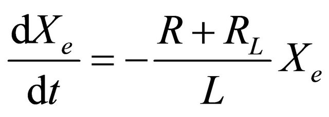In this case. It means that with step 0.001 s eigenvalues will be within the steel Rs area (see Figure 4).

The scheme RKM with reduction of state variable U_C shown in Figure 6 coincides at-a-glance with the analytical decision (Analyt), starting from the second point. The scheme of trapezia (Trap), with the chosen step, has the biggest margin of error, bigger, than the implicit Euler method (ImEuler).

5. Conclusion

This paper illustrates a possible reason why popular implicit schemes can produce results of questionable quality. According to the author a promising approach is the use of explicit schemes and the principle of reduction of the state variables, with pin-point use of implicit methods. The main advantage of explicit schemes is absence of need to solve a large system of linear equations at each integration step, which includes all the basic variables at once (for example, all the nodal potentials). It is at this stage, that the main CPU time is spent, additional errors appear, and, moreover, it is poorly parallelized.

6. Acknowledgements

Research work described in the article was completed within the Russian state assignment for year of 2012; project #7.2868.2011.

REFERENCES

- L. W. Nagel and D. O. Pederson, “Simulation Program with Integrated Circuit Emphasis,” Memorandum No. ERL-M382, University of California, Berkeley, 1973. http://en.wikipedia.org/wiki/SPICE
- Y. Tanovitskiy and D. A. Izotov, “A Mathematical Model of the Electronics Circuits for Analysis Chaos and Bifurcation Phenomena in the Pulse Power Systems,” Technichna Electodinamica. Tematichni Vipusk: Problemi Suchasnoy Electrotechniki, Vol. 7, 2004, pp. 80-85.
- E. Hairer and G. Wanner, “Solving Ordinary Differential Equations II: Stiff and Differential-Algebraic Problems,” 2nd Edition, Springer-Verlag, Berlin, 1996.
- R. H. Merson, “An Operational Method for the Study of Integration Processes,” Proceedings of Symposium on Data Processing, Weapons Research Establishment, Salisbury, 1957, pp. 110-125.
- I. S. Berezin and N. P. Zhidkov, “Computing Methods,” Pergamon Press, New York, 1973.
- R. Horn and C. Johnson, “Matrix Analysis,” Cambridge University Press, Cambridge, 1989.
- V. S. Baushev, Zh. T. Zhusubaliev and S. G. Mikhalchenko, “Stocastic Features in the Dynamic Characteristics of a Pulse-Width Controlled Voltage Stabilizer,” Electrical Techonology, Vol. 1, No. 3, 1996, pp. 137-150.