Applied Mathematics
Vol.3 No.8(2012), Article ID:21480,9 pages DOI:10.4236/am.2012.38129
On the Homotopy Analysis Method and Optimal Value of the Convergence Control Parameter: Solution of Euler-Lagrange Equation
Department of Applied Mathematics, School of Mathematical Sciences, Ferdowsi University of Mashhad, Mashhad, Iran
Email: *saberi hssn@yahoo.com
Received May 19, 2012; revised June 20, 2012; accepted June 27, 2012
Keywords: Homotopy Analysis Method; Calculus of Variations; Variational Problems; Euler-Lagrange Equation; Square Residual Error
ABSTRACT
This paper presents, an efficient approach for solving Euler-Lagrange Equation which arises from calculus of variations. Homotopy analysis method to find an approximate solution of variational problems is proposed. An optimal value of the convergence control parameter is given through the square residual error. By minimizing the square residual error, the optimal convergence-control parameters can be obtained. It is showed that the homotopy analysis method was valid and feasible to the study of variational problems.
1. Introduction
There has been a considerable renewal of interest in the classical problems of the calculus of variations both from the point of view of mathematics and of applications in physics, engineering, and applied mathematics. The direct method of Ritz and Galerkin in solving variational problems has been of considerable concern and is well covered in many textbooks [1-3]. Chen and Hsiao [4] introduced the Walsh series method to variational problems. Due to the nature of the Walsh functions, the solution obtained were piecewise constant. Razzaghi [5] applied the Fourier series, to derive a continuous solution for the second example in [4] which is an application to the heat conduction problem. Very recently, Dehghan and Tatari applied the Adomian decomposition method and variational iteration method to solve variational problems in [6,7], respectively and Abdulaziz, Hashim and Chowdhury applied the homotopy perturbation method to solve variational problems in [8].
One of the semi-exact methods for solving nonlinear Equation which does not need small/large parameters is HAM, first proposed by Liao in 1992 [9-13]. Since Liao [10] for the homotopy analysis method was published in 2003, more and more researchers have been successfully applying this method to various nonlinear problems in science and engineering, such as the viscous flows of non-Newtonian fluids [14], the KdV-type equations [15], finance problems [16], nonlinear optimal control problems [17] and so on.
The HAM contains a certain auxiliary parameter  which provides us with a simple way to adjust and control the convergence region and rate of convergence of the series solution. Moreover, by means of the so-called
  -curve, it is easy to determine the valid regions of
  to gain a convergent series solution. Thus, through HAM, explicit analytic solutions of nonlinear problems are possible. In this paper, we will adopt the homotopy analysis method (HAM), for solving the Euler-Lagrange equation, which arises from problems in calculus of variations.
2. Basic Idea of HAM
To describe the basic ideas of the HAM, we consider the following differential Equation
 (1)
(1)
where  is a nonlinear operator,
  denotes independent variable,
  is an unknown function, respecttively. For simplicity, we ignore all boundary or initial conditions, which can be treated in the similar way. By means of generalizing the traditional homotopy method, Liao [9] constructs the so-called zero-order deformation Equation
 (2)
(2)
where  is the embedding parameter,
  is a non-zero auxiliary parameter,
  is an auxiliary function,
  is an auxiliary linear operator,
  is an initial guess of
 ,
,  is a unknown function, respectively. It is important, that one has great freedom to choose auxiliary things in HAM. Obviously, when
  and
and , it holds
 (3)
(3)
respectively. Thus, as  increases from 0 to 1, the solution
  varies from the initial guess
  to the solution
 . Expanding
  in Taylor series with respect to
 , we have
 (4)
(4)
where
 (5)
(5)
If the auxiliary linear operator, the initial guess, the auxiliary parameter  and the auxiliary function are so properly chosen, the series (4) converges at
 , then we have
 (6)
(6)
which must be one of solutions of original nonlinear equation, as proved by Liao [10]. As  and
and , Equation (2) becomes
 (7)
(7)
which is used mostly in the homotopy perturbation method [18], where as the solution obtained directly, without using Taylor series. According to the definition (5), the governing equation can be deduced from the zero-order deformation Equation (2). Define the vector

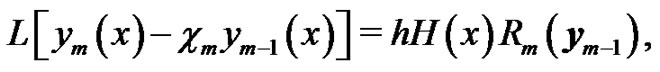
Differentiating Equation (2)  times with respect to the embedding parameter
  and then setting
  and finally dividing them by
 , we have the so-called
  th-order deformation Equation
 (8)
(8)
where
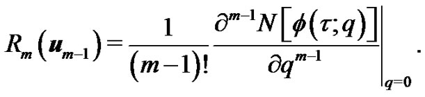 (9)
(9)
and
 (10)
(10)
It should be emphasized that  for
for  is governed by the linear Equation (8) under the linear boundary conditions that come from original problem, which can be easily solved by symbolic computation software such as Matlab. For the convergence of the above method we refer the reader to Liao’s work. If Equation (1) admits unique solution, then this method will produce the unique solution.
Remark 1. In 2007, Yabushita et al. [19] applied the HAM to solve two coupled nonlinear ODEs, and suggested the so-called optimization method to find out two optimal convergence-control parameters by means of the minimum of the square residual error integrated in the whole region having physical meanings. Their approach is based on the square residual error
 (11)
(11)
of a nonlinear Equation , where
  gives the
  th-order HAM approximation. Obviously,
  (as
(as ) corresponds to a convergent series solution. For given order
  of approximation, the optimal value of
  is given by a nonlinear algebraic equation

We use exact square residual error (11) integrated in the whole region of interest , at the order of approximation M.
3. Statement of the Problem
Let us consider the simplest form of the variational problems
 (12)
(12)
where  is the functional whose extremum must be found. In order to find the extreme value of
 , the boundary conditions of the admissible curves are given by
 (13)
(13)
The necessary condition for the solution to problem (12) is to satisfy the Euler-Lagrange equation:
 (14)
(14)
with the boundary conditions given in (13).
The boundary value problem (14) does not always have a solution and if the solution exists, it may not be unique. Note that in many variational problems the existence of a solution is obvious from the physical or geometrical meaning of the problem and if the solution of Euler’s Equation satisfies the boundary conditions, it is unique. Also this unique extremal will be the solution of the given variational problem.
The form of a variational problem involving two derivative can be considered as
 (15)
(15)
where  is the functional that its extremum must be found. To find the extreme value of
 , the boundary conditions of the admissible curves are known in the following form
 (16)
(16)
where  are known.
The necessary condition for the solution of the problem (15) is to satisfy the Euler-Lagrange Equation
 (17)
(17)
with boundary conditions given in (16).
The Euler-Lagrange equations (14), (17) are in general a nonlinear differential equation, which does not always have an analytic solution.
4. Numerical Results
To demonstrate the effectiveness of the HAM algorithm discussed above, several examples of variational problems will be studied in this section.
Example 4.1. We consider the following variational problem:
 (18)
(18)
subject to the boundary conditions
 (19)
(19)
The corresponding Euler-Lagrange Equation is given by
 (20)
(20)
subject to the boundary conditions (19).
To solve Equation (20) by means of HAM, we consider the following process after separating the linear and nonlinear parts of the equation.
From Equation (20), we define the nonlinear operator
 (21)
(21)
According to the initial condition denoted by (19), it is natural to choose

We choose the linear operator
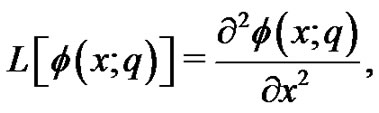 (22)
(22)
with the property , where
  are coefficient.
As mentioned in Section 2, we get the so-called  th-order deformation equation:
where

Now, the terms of the HAM solution can be given by

Hence, the solution to (20) is  which is the exact solution.
Example 4.2. We consider the following brachistochrone problem:
 (23)
(23)
subject to the boundary conditions
 (24)
(24)
The corresponding Euler-Lagrange Equation is given by
 (25)
(25)
with boundary conditions (24). The exact solution to the brachistochrone problem (23) in implicit form is

Following Zhang and He [20], we can expand the nonlinear term  in (25) using the Taylor series as follows:

Hence, we can rewrite the Euler-Lagrange Equation (25) as follows:
 (26)
(26)
To solve Equation (26) by means of HAM, we define the nonlinear operator

From the initial conditions (24), the initial guess is

As mentioned in Section 2, we get the so-called  th-order deformation equation with

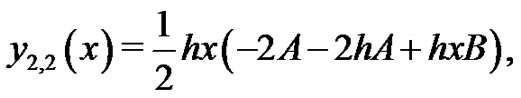
Now, the terms of the HAM solution can be given by

In Figures 1-4, we plot the comparison of error function  for
for  with
with . Figure 5 shows the 4-term HAM approximate solution
  of (26). When
 , it is easily seen that the solutions above are exactly the solutions in [8]. Therefore, the HPM solution is indeed a special case of the HAM solution when
 .
.
By HAM, it is easy to discover the valid region of h, which corresponds to the line segments nearly parallel to the horizontal axis. To find a proper value of  the
the  - curve of
  given by the 8th-order HAM appro-

Figure 1. Error function (h = –1, h = –0.9).

Figure 2. Error function (h = –1, h = –0.8).

Figure 3. Error function (h = –1, h = –0.8).
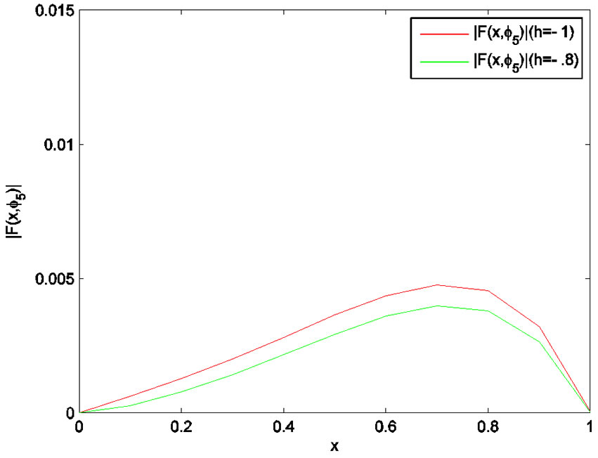
Figure 4. Error function (h = –1, h = –0.8).

Figure 5. The 4th-order HAM results.
ximation is drawn in Figure 6, which clearly indicates that the valid region of  is about
 .
.
As mentioned in Section 2, the optimal value of  is determined by the minimum of
 , corresponding to the nonlinear algebraic Equation
 . Our calculations showed that,
  has its minimum value at –0.9.
Example 4.3. We consider the following variational problem:
 (27)
(27)
subject to the boundary conditions
 (28)
(28)
The corresponding system of Eulers differential equations is given by
 (29)
(29)

Figure 6. The h-curve of y(0.1) 8th-order HAM.
with boundary conditions (28). The exact solution to the variational problem (27) is as follows [6]:

To solve the Equations (29) by means of homotopy analysis method, we choose the initial guess
 (30)
(30)
We now define a nonlinear operators as:

As mentioned in Section 2, we get the so-called  thorder deformation Equation with

and initial conditions:

We start with an initial approximation  we can obtain directly the other components as:


Imposing the boundary conditions on  and
and , we obtain
 . Hence with
 , the exact solution of the problem will be obtained. In Figures 7 and 8, we compare the exact solution
  with the 2-term HAM approximate solution, for
 . Figures 9 and 10 shown the
  -curve of
  given by the 8th-order HAM approximation.
As mentioned in Section 2, the optimal value of  is determined by the minimum of
 , corresponding to the

Figure 7. Comparison between the HAM solution of y(x) and the exact solution.

Figure 8. Comparison between the HAM solution of z(x) and the exact solution.

Figure 9. The h-curve of .
.

Figure 10. The h-curve of .
.
nonlinear algebraic Equation . Our calculations showed that,
  has its minimum value at
 .
.
Example 4.4. In this example we consider the variational problem
 (31)
(31)
subject to the boundary conditions
 (32)
(32)
which has the the exact solution .
.
The Euler-Lagrange Equation of this problem can be written in the following form
 (33)
(33)
Applying the homotopy analysis method for solving this problem,we consider the transformation

we rewrite the above fourth-order boundary value problem as a system of differential equations
 (34)
(34)
 (35)
(35)
 (36)
(36)
 (37)
(37)
To solve Equations (34)-(37) by means of the HAM, we choose the initial approximations
 (38)
(38)
Furthermore, we define a system of nonlinear operators as

As mentioned in Section 2, we get the so-called  thorder deformation Equation with

We start with an initial approximation, we can obtain directly the other components as:


when , it is easily seen that the solutions above are exactly the solutions in [6],

Imposing the boundary condition on  we have

In Figure 11, we compare the exact solution  with the 10-term HAM approximate solution, and also the numerical results can be seen in Table 1.
As mentioned in Section 2, the optimal value of  is determined by the minimum of
 , corresponding to the nonlinear algebraic Equation
 . Our calculations showed that,
  has its minimum value at
 .
.
5. Conclusion
In this paper, we have successfully developed HAM for solving variational problems. It is apparently seen that HAM is a very powerful and efficient technique in finding analytical solutions for wide classes of linear and nonlinear problems. By minimizing the the square residual error, the optimal convergence-control parameters

Figure 11. Comparison between the 10-term HAM solution and the exact solution.

Table 1. The result of the HAM for n = 7 and h = –1.
obtained. The results got from the performance of HAM over variational problems, was specified that the solution of HAM in special case is similar to numerical results of HPM, VIM and ADM.
REFERENCES
- I. M. Gelfand and S. V. Fomin, “Calculus of Variations,” Prentice Hall, New Jersey, 1963.
- L. Elsgolts, “Differential Equations and the Calculus of Variations,” Mir Publisher Moscow, 1977.
- L. Elsgolts, “Calculus of Variations,” Pergamon Press, Oxford, 1962.
- C. F. Chen and C. H. Hsiao, “A Walsh Series Direct Method for Solving Variational Problems,” Journal of the Franklin Institute, Vol. 300, No. 4, 1975, pp. 265-280. doi:10.1016/0016-0032(75)90199-4
- M. Razzaghi and M. Razzaghi, “Fourier Series Direct Method for Variational Problems,” International Journal of Control, Vol. 48, No. 3, 1988, pp. 887-895. doi:10.1080/00207178808906224
- M. Dehghan and M. Tatari, “The Use of Adomian Decomposition Method for Solving Problems in Calculus of Variations,” Mathematical Problems in Engineering, 2006, pp. 653-679.
- M. Tatari and M. Dehghan, “Solution of Problems in Calculus of Variations via He’s Variational Iteration Method,” Physics Letters A, Vol. 362, No. 5-6, 2007, pp. 401-406. doi:10.1016/j.physleta.2006.09.101
- O. Abdulaziz, I. Hashim and M. S. H. Chowdhury, “Solving Variational Problems by Homotopy Perturbation Method,” International Journal for Numerical Methods in Engineering, Vol. 75, No. 6, 2008, pp. 709-721. doi:10.1002/nme.2279
- S. J. Liao, “The Proposed Homotopy Analysis Technique for the Solution of Nonlinear Problems,” Ph.D. Thesis, Shanghai Jiao Tong University, Shanghai, 1992.
- S. J. Liao, “Beyond Perturbation: Introduction to the Homotopy Analysis Method,” CRC Press, Chapman & Hall, Boca Raton, 2003.
- S. J. Liao, “On the Homotopy Anaylsis Method for Nonlinear Problems,” Applied Mathematics and Computation, Vol. 147, No. 2, 2004, pp. 499-513. doi:10.1016/S0096-3003(02)00790-7
- S. J. Liao, “Comparison between the Homotopy Analysis Method and Homotopy Perturbation Method,” Applied Mathematics and Computation, Vol. 169, No. 2, 2005, pp. 618-634. doi:10.1016/j.amc.2004.10.058
- S. J. Liao, “Homotopy Analysis Method: A New Analytical Technique for Nonlinear Problems,” Communications in Nonlinear Science and Numerical Simulation, Vol. 2, No. 2, 1997, pp. 95-100. doi:10.1016/S1007-5704(97)90047-2
- T. Hayat, T. Javed and M. Sajid, “Analytic Solution for Rotating Flow and Heat Transfer Analysis of a ThirdGrade Fluid,” Acta Mechanica, Vol. 191, No. 3-4, 2007, pp. 219-229. doi:10.1007/s00707-007-0451-y
- S. Abbasbandy, “Soliton Solutions for the 5th-Order KdV Equation with the Homotopy Analysis Method,” Nonlinear Dynamics, Vol. 51, No. 1-2, 2008, pp. 83-87. doi:10.1007/s11071-006-9193-y
- S. P. Zhu, “An Exact and Explicit Solution for the Valuation of American Put Options,” Quantitative Finance, Vol. 6, No. 3, 2006, pp. 229-242. doi:10.1080/14697680600699811
- S. Effati and H. Saberi Nik, “Analytic-Approximate Solution for a Class of Nonlinear Optimal Control Problems by Homotopy Analysis Method,” Asian-European Journal of Mathematics, in press.
- J. H. He, “Homotopy Perturbation Technique,” Computer Methods in Applied Mechanics and Engineering, Vol. 178, No. 3-4, 1999, pp. 257-262. doi:10.1016/S0045-7825(99)00018-3
- K. Yabushita, M. Yamashita and K. Tsuboi, “An Analytic Solution of Projectile Motion with the Quadratic Resistance Law Using the Homotopy Analysis Method,” Journal of Physics A, Vol. 40, No. 29, 2007, pp. 8403- 8416. doi:10.1088/1751-8113/40/29/015
- L. N. Zhang and J. H. He, “Homotopy Perturbation Method for the Solution of the Electrostatic Potential Differential Equation,” Mathematical Problems in Engineering, 2006, pp. 838-848.
NOTES
*Corresponding author.