Applied Mathematics, 2011, 2, 1170-1174
doi:10.4236/am.2011.29162 Published Online September 2011 (http://www.SciRP.org/journal/am)
Adaptive Control of a Production-Inventory Model
with Uncertain Deterioration Rate
Fawzy Bukhari
Department of St ati s ti c s and Oper at i o ns Research, College of Science, King Saud University, Riyadh, Saudi Arabia
Received July 6, 2011; revised July 22, 2011; accepted July 29, 2011
Abstract
This paper studied a continuous-time model of a production maintenance system in which a manufacturing
firm produces a single product selling some and stocking the remaining. The problem of adaptive control of
a production-maintenance system with unknown deterioration has been presented. Using Liapunov technique,
the production rate and updating rule of deterioration rate are derived as non-linear functions of inventory
level perturbation. Numerical analysis for the system has been presented for a set of parameter values and
demand rate.
Keywords: Production Inventory System, Adaptive Control, Liapunov Technique
1. Introduction
Applications of optimal control theory to management
science, in general, and to production planning, in par-
ticular, are proving to be quite fruitful; see for example
Sethi and Thompson [1]. Naturally, with the optimal
control theory, optimal control techniques came to be
applied to production planning problems and others. For
example, Dobos [2] have discussed the problem of a re-
verse logistics system with special structure. The prob-
lem was presented as an optimal control problem with
two state variables and with three control variables with
an objective to minimize the sum of the quadratic devia-
tion from the goal values. Nahmias [3], Porter and Taylor
[4], Raafat [5], and Khemlnitsky and Gerchak [6] have
discussed the problems of production inventory systems
with inventory levels dependant on demand rate, the
problem of modal control of production inventory sys-
tems, and inventory systems with deteriorating items.
Caldwell [7], Aseltine, Mancini and Sartune [8], Landau
[9], and Narendra and Annaswamy [10] have solved
many problems by using the adaptive control of linear
and non linear dynamical systems using a feedback ap-
proach. El-Gohary and Al-Ruzaiza [11] have studied the
adaptive control of a continuous time three species prey
predator populations. They have derived the nonlinear
feedback control inputs asymptotically stabilized the
system about its steady states. El-Gohary and Yassen [12]
have used the adaptive control and synchronization pro-
cedures to the coupled dynamo system with unknown
parameters. Based on the Liapunov stability technique,
an adaptive control laws are derived such that the cou-
pled dynamo system is asymptotically stable and the two
identical dynamo systems are asymptotically synchro-
nized. Also, the update rules of the unknown parameters
are derived. Tadj, Sarhan and El-Gohary [13] have dis-
cussed the optimal control of an inventory system with
ameliorating and deteriorating items. Different cases for
the difference between the ameliorating and deteriorating
items are considered. Foul, Tadj, and Hedjar [14] have
studied the problem of adaptive control of a production
inventory system in which a manufacturing firm pro-
duces a single product selling some and stocking the re-
maining. Model reference adap tive co ntrol with feedb ack
is applied to track the output of the system toward the
inventory goal level.
The paper studies a production-inventory model which
produces a single item with a certain production rate and
seeks an adaptive actual production and inventory rates.
This model has a dynamic nature and an adaptive control
approach seems particularly well suited to achieve its
goal level and production rate. Also, the unknown dete-
rioration rate will be derived from the conditions of as-
ymptotic stabilization about the steady-state.
The rest of the paper is organized as follows. Follow-
ing this introduction, the mathematical model is intro-
duced in Section 2. In Section 3, the problem of adaptive
control of the production inventory system with un-

F. BUKHARI1171
known deterioration rate is discussed. Also the desired
production rate and updating rule of the deterioration rate
are derived from the conditions of the asymptotic stabil-
ity of the system. In Section 4, we present some illustra-
tive examples. The numerical solution of the controlled
model is presented. Section 5 presents a conclusion of
the paper.
2. Mathematical Model
Consider a manufacturing system that produces a single
product, selling some units and adding others to inven-
tory. We start by writing the differential equation mod-
els. These can be conveniently formulated in terms of
Moreover, the following variables and parameters are
used:
()
I
t()Pt : the inventory level at time t,
a()Dt : the actual production rate at time t,
: the demand rate at time t,
()ut : the desired production rate at time t,

: the deterioration rate,

: the inverse of exponential delay time,
I: the inventory level at the steady state,
a
P: the actual production rate at steady state,
D: the demand rate at steady state.
All functions are assumed to be nonnegative, continu-
ous and differentiable. Assume that at the time instant t
the demand occurs at rate , the actual production at
rate , and the actual production rate responds to
the desired production rate with an exponential
time-delay of
()Dt
()
a
Pt
1

, it follows that the inventory level
()
I
t and the actual production rate evolve ac-
cording to the following first order differential equa-
tions:
()
a
Pt
ˆ
()() ()()(),
()() (), ()
a
aa
I
tPt tItDt
PtutPt



 


 


(1)
where, the “dot” means the differentiation with respect to
time and the initial state is0 (0)
I
I, a . This
balance equations were also used by Porter and Taylor
(1972), Bradshaw and Porter (1975), and Riddalls and
Bennett (2001) without deterioration rate
(0)
a
PP

. The
steady-states of this system can be derive by setting both
()
I
t
 and equal to zero. That is: ()
a
Pt


1,
a
I
pD 


a
pu (2)
Next, in what follows we will discuss the adaptive
control of the produ ction inventory model with unknown
deterioration rate using Liapunov technique.
3. Adaptive Control Problem
In this section, we will discuss in details the adaptive
control problem of the reference model. The rates of de-
mand and desired production, and updating rule of dete-
rioration rate will be derived from the condition of as-
ymptotic stability of the reference model. To study the
adaptive control p roblem we start by considering the val-
ues of required inventory goal level, and actual produc-
tion goal rate as the steady-state solution of the reference
model Equation (1). We consider the adaptive system as
follows:
ˆ
()() ()()(),
()() (), ()
a
aa
I
tPt tItDt
PtutPt



 


 


(3)
where, ˆ()t

is the dynamic estimator of the unknown
deterioration rate

. Following, we assume that ()
I
tI

,
()
aa
Pt P

, ()ut u

, ()Dt D, and ˆ()t

  is a spe-
cial solution for the system Equation (3). The equations
of perturbed states of the reference system about its
steady states can be derived by introducing the following
new variables:
12
()(), ()(),
ˆ
()(),()(), ()(),
aa
tItI tPtP
vtutudtDtDtt



  


 

 (4)
Substituting from Equation (4) into Equation (3) we
get the following perturbed system:
121 1
22
()()() ()()()(),
()()(),
[]
tttt tItdt
tvtt
 
 

 



 


(5)
The system Equation (5) will be used to study the
adaptive control problem using the Liapunov technique
for the system of Equation (4). The following theorem
gives the desired production rate and updating rule for
deterioration rate ensure the asymptotic stability of the
reference production inventory model with uncertain
deterioration rate.
Theorem 1
If the perturbations of both desired production rate and
updating rule o f the deterioration rate are giv e n by :


12
()() ()vttkt

    (6)
and
2
11
() ()()()ttItmt

  
 (7)
where, k, and m are positive real control gains parameters.
Then the special solution () 0,(1,2)
iti

, () 0vt

,
and () 0t


of the systems Equations (5) and (7) is

F. BUKHARI 1172
t
asymptotically stable in Liapunov sense if the demand
rate is linear function of the perturbation of the inventory
level or the actual production rate. Otherwise, the as-
ymptotic stability of the solution requires further mathe-
matical analysis.
Proof: The proof of this theorem based on the selec-
tion of a suitable Liapunov function for the system con-
sists of the two combined systems Equations (5) and
(7).
Assume this function has the form:

2
22
12 1
, ,()()
ii
t  


 (8)
This function is a positive definite function of the
variables (),( 1,2)
iti

, and ()t

. The total time de-
rivative of the Liapunov function Equation (8) along the
trajectory of the systems Equations (5) and (7) give:
222
12
()()()()() ()[]tktmtdt    
1
t (9)
Since 0k


() ()
ft t
,, the sign of depends
upon the perturbation of the demand rate. In this paper,
we will consider the following two possibilities which
are: 1
0m 

()dt

 or 2 ()() ()dt gtt


. Hence, the
total time derivative of the Liapunov function takes the
form:
222
12
222
12 1
(()) ()() ()(),
()()()()() ()(),
fttkt mt
tktmtgtt

 
 


 


2
t
(10)
So, the special solution: () 0,(1,2)
iti

, ()0vt

,
and () 0t

 is asymptotically stable in the Liapunov
sense if: 2( )
g
k   which comp letes th e proof.
Now, substituting the adaptive controlled desired pro-
duction rate and updating rule of the deterioration rate
Equation (5) into Equation (4) we get the following con-
trolled system:
121 1
2122
2
11
()()() ()()()(),
()() ()(),
()() ()(),
tttt tItdt
ttktt
tIttmt
 

 

 



 







(11)
The above system is used to study the time evolution
of inventory levels and dynamic estimators of deteriora-
tion rates. It appears from Equation (11) that the analyti-
cal solution of the system is difficult to derive since it is
non-linear and therefore we solve it numerically in the
next section.
4. Numerical Solution
The objective of this section is to study the numerical
solution of the problem to determine an adaptive control
strategy for a produ ction inventory model with unknown
deterioration rate. The numerical solution algorithm is
based on numerical integration of the system using the
Runge-Kutta method. This section displays graphically
the numerical integration of system Equation (11) of
differential equations for a set of parameter values.
4.1. Example 1
In this example we will graphically display the system
behavior subjected to linear demand rate of the inventory
perturbation. The following set of parameter values is
assumed:
Parameter kmf

I

Value 332 0.05 50 0.2
With the following values of initial perturbations of
inventory level, actual production rate, and deterioration
rate: 1(0) 40


, 2(0)15


, (0) 0.02

 respectively.
The numerical results are illustrated in Figures 1(a)-(d)
as follows:
Figures 1(a)-(c) have indicated that both the perturba-
tions of inventory level and deterioration rate are damp-
ing oscillate about their goal values. While Figure 1(b)
indicates that the actual production rate perturbation ex-
ponentially tends to its goal value. Finally, Figure 1(d)
shows that the desired production rate exponentially os-
cillates about its goal value.
4.2. Example 2
In this example we will graphically display the system
behavior subjected to linear demand rate of the actual
production rate perturbation. The following set of pa-
rameter values is assumed:
Parameter k m f

I

Value 0.050.010.2 0.05 200 5
With the following values of initial perturbations of
inventory level, actual production rate, and deterioration
rate: 1(0) 50


, 2(0)15


, (0) 0.02

 respectively.
The numerical results are illustrated in Figures 2(a)-(d)
as follows:
Figures 2(a)-(d) have indicates that the perturbations of
inventory level, deterioration rate, and desired production
rate are damping oscillate about their goal values. While
Figure 2(b) indicates that the actual production rate per-
turbation exponen tially tends to its goal value.

F. BUKHARI 1173
40
30
20
10
0
-10
-20
-30
0.5 1 1. 5 2
T
ξ
1
(a) (b)
(c) (d)
Figure 1. (a) Perturbation of inventory level; (b) Perturbation of actual production rate; (c) Perturbation of deterioration
rate; (d) Perturbation of desired production rate.
(a) (b)

F. BUKHARI 1174
(c) (d)
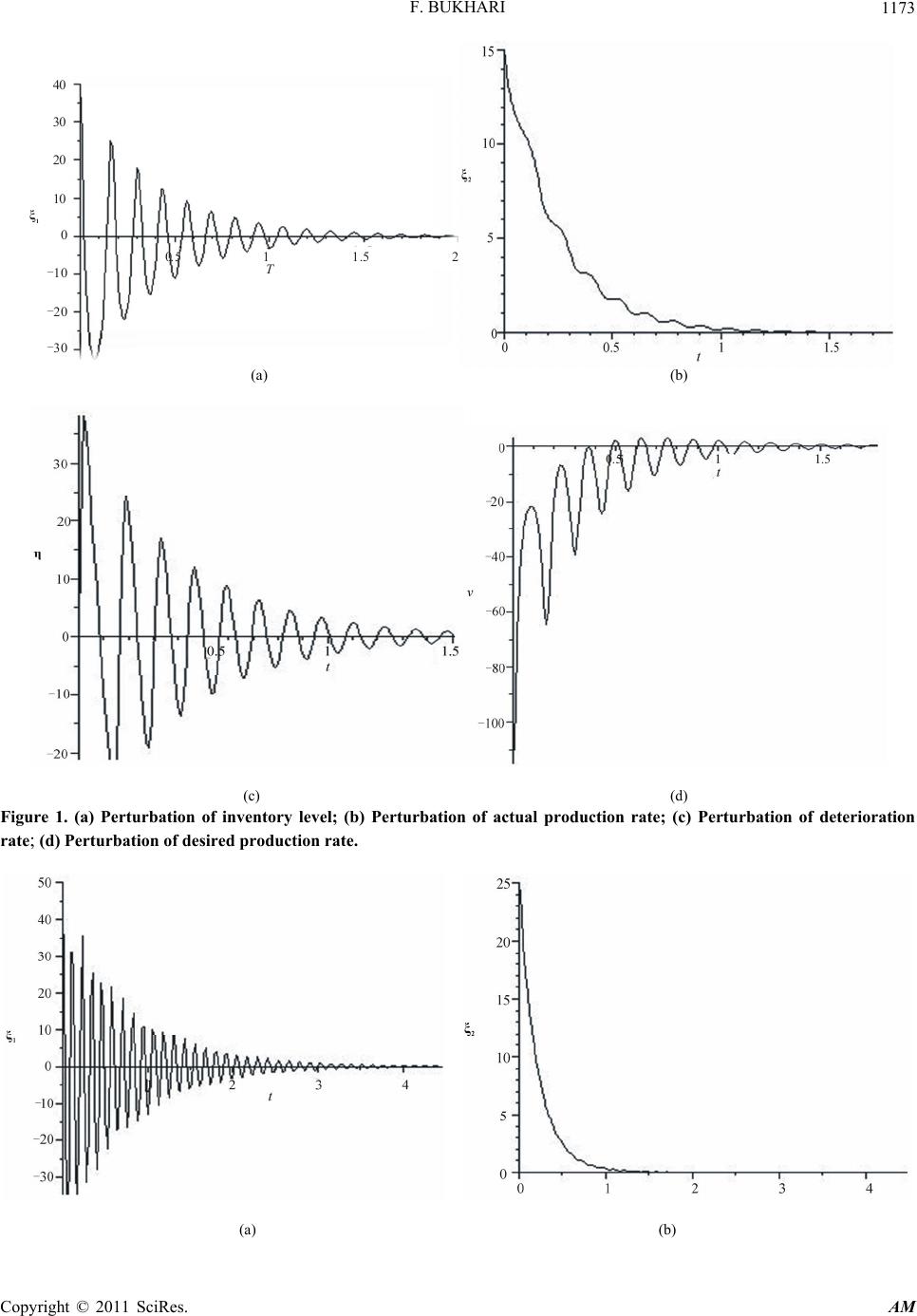
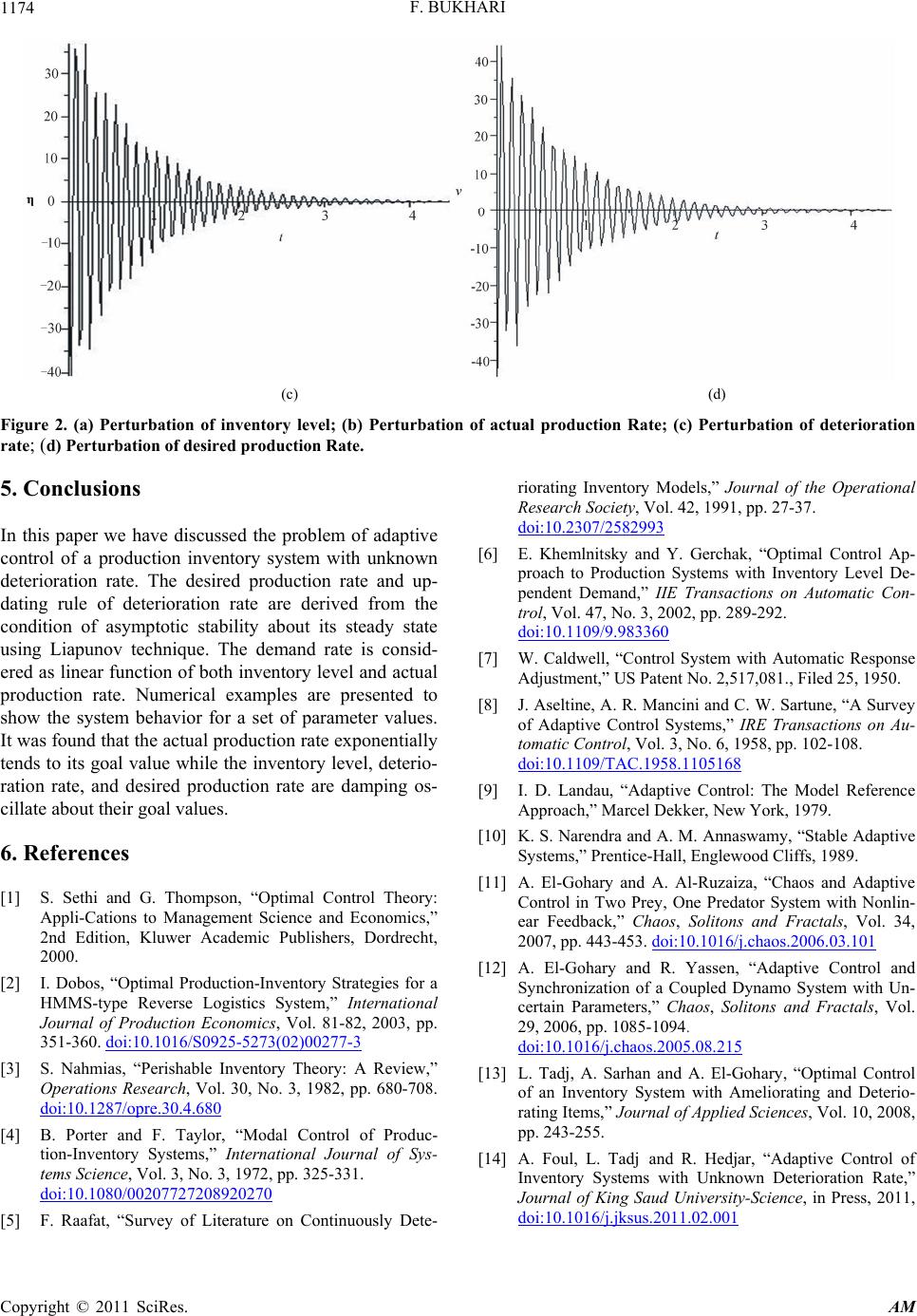
Figure 2. (a) Perturbation of inventory level; (b) Perturbation of actual production Rate; (c) Perturbation of deterioration
rate; (d) Perturbation of desired production Rate.
5. Conclusions
In this paper we have discussed the problem of adaptive
control of a production inventory system with unknown
deterioration rate. The desired production rate and up-
dating rule of deterioration rate are derived from the
condition of asymptotic stability about its steady state
using Liapunov technique. The demand rate is consid-
ered as linear function of both inventory level and actual
production rate. Numerical examples are presented to
show the system behavior for a set of parameter values.
It was found that the actual production rate exponentially
tends to its goal value while the inventory level, deterio-
ration rate, and desired production rate are damping os-
cillate about their goal values.
6. References
[1] S. Sethi and G. Thompson, “Optimal Control Theory:
Appli-Cations to Management Science and Economics,”
2nd Edition, Kluwer Academic Publishers, Dordrecht,
2000.
[2] I. Dobos, “Optimal Production-Inventory Strategies for a
HMMS-type Reverse Logistics System,” International
Journal of Production Economics, Vol. 81-82, 2003, pp.
351-360. doi:10.1016/S0925-5273(02)00277-3
[3] S. Nahmias, “Perishable Inventory Theory: A Review,”
Operations Research, Vol. 30, No. 3, 1982, pp. 680-708.
doi:10.1287/opre.30.4.680
[4] B. Porter and F. Taylor, “Modal Control of Produc-
tion-Inventory Systems,” International Journal of Sys-
tems Science, Vol. 3, No. 3, 1972, pp. 325-331.
doi:10.1080/00207727208920270
[5] F. Raafat, “Survey of Literature on Continuously Dete-
riorating Inventory Models,” Journal of the Operational
Research Society, Vol. 42, 1991, pp. 27-37.
doi:10.2307/2582993
[6] E. Khemlnitsky and Y. Gerchak, “Optimal Control Ap-
proach to Production Systems with Inventory Level De-
pendent Demand,” IIE Transactions on Automatic Con-
trol, Vol. 47, No. 3, 2002, pp. 289-292.
doi:10.1109/9.983360
[7] W. Caldwell, “Control System with Automatic Response
Adjustment,” US Patent No. 2,517,081., Filed 25, 1950.
[8] J. Aseltine, A. R. Mancini and C. W. Sartune, “A Survey
of Adaptive Control Systems,” IRE Transactions on Au-
tomatic Control, Vol. 3, No. 6, 1958, pp. 102-108.
doi:10.1109/TAC.1958.1105168
[9] I. D. Landau, “Adaptive Control: The Model Reference
Approach,” Marcel Dekker, New York, 1979.
[10] K. S. Narendra and A. M. Annaswamy, “Stable Adaptive
Systems,” Prentice-Hall, Englewood Cliffs, 1989.
[11] A. El-Gohary and A. Al-Ruzaiza, “Chaos and Adaptive
Control in Two Prey, One Predator System with Nonlin-
ear Feedback,” Chaos, Solitons and Fractals, Vol. 34,
2007, pp. 443-453. doi:10.1016/j.chaos.2006.03.101
[12] A. El-Gohary and R. Yassen, “Adaptive Control and
Synchronization of a Coupled Dynamo System with Un-
certain Parameters,” Chaos, Solitons and Fractals, Vol.
29, 2006, pp. 1085-1094.
doi:10.1016/j.chaos.2005.08.215
[13] L. Tadj, A. Sarhan and A. El-Gohary, “Optimal Control
of an Inventory System with Ameliorating and Deterio-
rating Items,” Journal of Applied Sciences, Vol. 10, 2008,
pp. 243-255.
[14] A. Foul, L. Tadj and R. Hedjar, “Adaptive Control of
Inventory Systems with Unknown Deterioration Rate,”
Journal of King Saud University-Science, in Press, 2011,
doi:10.1016/j.jksus.2011.02.001