ABSTRACT

In presented paper we try to consider problems of the gravitational optics and dark matter developing from the crystal model for the vacuum. How it is follows from consideration it enables to describe both electromagnetic waves and spectrum of elementary particles from the unified point of view. Two order parameters – a polar vector and an axial vector - had to be introduced as electrical and magnetic polarization, correspondingly, in order to describe dynamic properties of vacuum. Vacuum susceptibility has been determined to be equal to the fine structure constant a . Unified interaction constant g for all particles equal to the double charge of Dirac monopole has been found (g = e/a, where e charge electron). The fundamental vacuum constants are: g, a, parameters of  length and parameters of time for electron and nucleon oscillations, correspondingly. Energy of elementary particles has been expressed in terms of the fundamental vacuum parameters, light velocity being equal to. The term mass of particle has been shown to have no independent meaning. Particle energy does have physical sense as wave packet energy related to vacuum excitation. Exact equation for particle movement in the gravitational field has been derived, the equation being applied to any relatively compact object: planet, satellite, electron, proton, photon and neutrino. The situation has been examined according to the cosmological principle when galaxies are distributed around an infinite space. In this case the recession of galaxies is impossible, so the red shift of far galaxies’ radiation has to be interpreted as the blue time shift of atomic spectra; it follows that zero-energy, and consequently electron mass are being increased at the time. Since physical vacuum has been existed eternally, vacuum parameters can be either constant, or oscillating with time. It is the time oscillation of the parameters that leads to the growth of electron mass within the last 15 billion years and that is displayed in the red shift; the proton mass being decreased that is displayed in planet radiation.

1. Introduction

The science about cosmology has been in rather difficult situation in recent years. On one hand, observations of star dynamics in galaxies and of galaxies in clasters show substantial deviation of rotation velocities from Kepler’s law; this proves the existence of additional matter (dark matter) which participates in gravitational interaction [1- 3]. On the other hand, more careful examination of the red shift in the nearer space at the distances of 10⁵-10⁷ light years as well as observation of supernova outburst [4,5] show that velocity of the Universe expansion increases with time, and this in turn requires introduction of additional dark energy with anti-gravitational properties.

Thus, a contradiction arises. Practically, in one and the same point it is necessary to introduce both dark matter creating additional gravitational field and dark energy having anti-gravitation. Since there is no doubt about the facts above, their interpretation must be revised.

At the present time there are two mutually exclusive points of view. First, despite very distinctive spatial nonhomogeneity of matter, observations show that at the distances of about 10⁹ light years (cell of homogeneity) matter is distributed in the space quite homogeneously. Besides, the cosmological principle suggests that these homogeneous cells should cover the entire infinite space. Second, the red shift discovered by Hubble, which he interpreted as Doppler's principle related to the galaxies expansion, made Friedman’s model of expanding Universe quite necessary. From Hubble’s empirical law that determines dependence of velocity of galaxies on the distance v = Hr, we can suppose existence of a singularity at a certain time. Since velocity of expansion of the galaxies cannot exceed the light velocity c, it follows from the relation c = HR = HcT₀, that there is quite a definite size of the Universe growing with time R = cT₀, here –T₀ is the singularity offset counted from the present moment; Hubble’s constant equal to H = 1/T₀ decreases with time; however, observations show, that the value H, on the contrary, increases with time.

If we interpret the existence of a singularity as a Big Bang, we have to bear in mind that the explosion is a phase transition from a metastable state into another more stable state accompanied with release of energy. Before the phase transition, this energy is homogeneously distributed around the space. They sometimes say: explosion power is equivalent to e.g. one kilogram of trotyl; it is obvious that two kilograms of trotyl give off right twice as much energy as one kilogram does. Besides, the phase transition does not begin with the singularity but with the nucleation of a new phase whose size exceeds the critical radius. In this case energy is released in accordance with broadening the new phase at the expense of the phase edge motion. Since the average energy density of the entire matter in vacuum is approximately 0.008 erg/m³, this very energy should be released at the phase transition of each cubic meter of vacuum. It is difficult to imagine, however, that electrons and protons could be created out of this homogeneously distributed in space energy, and, besides, in exactly equal quantities. An explosion of a hydrogen bomb in vacuum can serve as a model of a hot Universe. The hydrogen bomb is a local object in a metastable state. There is a mixture of light and heavy nuclei under the temperature of several million degrees at the moment of detonation. According to D’Alambert equation, the electromagnetic pulse and the neutrino pulse will start to disperse with the light velocity. Following electromagnetic pulse relativistic electrons will fly and then light, and heavy nuclei. In a second, the electromagnetic pulse will reach the Moon area and nothing will stay at the point of explosion. Thus, the examined case is also far from the Friedman’s model of expanding Universe.

In order to somehow reconcile the model of the infinite matter distribution in space with that of the expanding Universe, Milne offered the following reasoning [6]. If we mentally specify a sphere of a definite size in a matter homogeneously distributed around an infinite space, then external layers of the sphere due to their spherical symmetry have no influence on the sphere dynamics. Therefore, we can ignore the external layers and consider the Universe as a sphere of a definite size that precisely coincides with the Friedman’s model. However, this statement is a mistake. The thing is that with matter being homogeneously distributed about the entire infinite space, the gravitational potential follows the condition of the translational invariance:. We may consider this constant to be equal to zero, therefore, a gravitational potential only arises at deviation of a matter distribution from an average value. For that reason the equation for the potential can be written as follows:

. (1)

Here is an average density of matter. From equation (1) we can see that it is not necessary to search for dark energy as the density is both the gravitating and the anti-gravitating matter in the form of and.

On the other hand, if we mentally specify a sphere of radius R with the density of matter and ignore the external matter, we come to another equation for the potential:

This equation has the following solutions:

(2)

Similar expressions can be used for determining gravitational potentials of planets, stars and galaxies in a form of the sum of the potentials of stars with their specific location. However, for the scales comparable with the size of homogeneity cell and bigger, we come to an obviously non-physical result: the potential in any arbitrary point depends on the radius of a sphere which we mentally specify out of the entire infinite space. Thus, any result depending on the mentally specified radius of the sphere, including the radius of the visible part of the Universe, is physically incorrect.

For instance, we can determine the circular orbital velocity v₁ for the Universe of radius R on the sphere surface from the equality of centripetal and centrifugal forces:

If v₁ is equal to the light velocity с, we obtain the following expression for the critical matter density in the Universe:

This corresponds to the condition R = r_g when r_g is a gravitational radius. Therefore, with the definite choice for R we may come to the conclusion that the Universe is a black hole, while, as it follows from the cosmological principle at the scales comparable with the radius of the visible part of the Universe, the gravitational potential has no specific features and its average value is zero.

The same situation takes place when we consider the influence of a pressure on the dynamics of the expanding Universe. For instance, if we take a big vessel with a gas, mentally specify a sphere of radius R in it, and ignore the gas surrounding the sphere, we can state that the gas will broaden and get cool at the expense of the internal pressure. This may remind the model of the expanding Universe. Remember, however, that the specified sphere is surrounded with the same gas at the same pressure; that is why there will be neither broadening nor cooling. Thus, for the infinite Universe both an average gravitational potential and an average pressure are constant; besides, since the expanding dynamics is influenced by the equal to zero gradients of these variables, there cannot be neither expanding nor compression. An infinite system can only stratify according to the energy density and we really observe this stratification on giant scales from the value less than 10^-9erg/cm³ for an inter-galaxy space to the value over 10³⁹ erg/cm³ for nuclear energy.

Nevertheless, within the frames of the cosmological principle there is a problem, the so called photometric paradox. The thing is that at present time when stars and galaxies radiate light in the entire infinite space, we can introduce an average luminosity L of a unit volume, provided that the densities of a luminous flux intensity at the distance r from a single volume is equal to j = L/4πr². The integral over the sphere of radius R gives the total flux intensity equal to J = RL; it follows that with R approaching infinity the flux intensity must approach infinity as well. Practically, however, we see rather a low sky luminosity. This is the photometric paradox.

In fact, by calculating the intensity, we must take into consideration the retardation effects. The flux that comes to a certain point (r = 0) at a certain time (t = 0) radiates at different moments depending on the distance:

(3)

Expression (3) shows that the flux coming from the deep Universe will be finite if L(t) at longer t decreases faster than 1/t.

Besides, we can divide the entire flux observed at any point of the infinite space into two parts: the flux J_vis of a visible part of space R = cT₀, Т₀ ~ 15·10⁹ years and the relict flux J_rel radiating from the spots with r > R:

Here summing was carried out over a countable number of galaxies in the visible part of the Universe. Thus, from the expressions given above it follows that the Universe must be non-stationary, not due to an expansion of galaxies’, but at the expense of a variation of physical vacuum parameters. Since the relict radiation corresponds to the temperature 3⁰K, the Universe had such a temperature long ago. The one but not the only feature of a non-stationarity is the red shift of atomic spectra that we can interpret as the blue temporal shift of both characteristic Bohr energy and all atomic energy levels correspondingly, at the expense of variation of physical vacuum parameters. Observations show that the characteristic Bohr frequency depends on time and increases with time. By introducing a frequency of an arbitrary atomic level, we obtain the following expression for the Hubble’s constant:

(4)

Both ω(t) and H(t) are monotonously increasing functions. The latest observations of the flashes of far supernova [4-5] show temporal growth of H. It is senseless to explain this situation using space-time properties.

Speaking about space-time properties is quite the same as judging about wine quality by the curvature of a bottle surface. Dilettantes are often attracted by the appearance of the vessel, while connoisseurs pay attention to its contents, conservation conditions, and temporal changes. We should regard space like a vessel with the only feature: its volume is infinite. Its internal properties are to be discussed.

2. Hidden Parameters of Vacuum

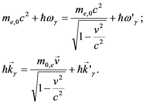
We should proceed from the experimental fact that the energy and the pulse of any elementary particle are:

(5)

Here ω_k-frequency for electron, proton, photon and neutrino, correspondingly, we expressed as follows:

(6)

The unified formula for the energy of any elementary particle points to the existence of the universal interaction for fields related to each particle. Besides, the two oscillation branches with the energy gap observed in the excitation spectrum prove an existence of a certain set of discrete oscillators whose interaction causes normal oscillations with frequencies ω_k. In fact, we can represent vacuum as a crystal object of a cubic or hexagonal symmetry with a very small lattice period, much less than 10^{-26 cm}. We can estimate the upper limit of a lattice period by the maximum particle energy in cosmic rays equal to 10²¹ eV that corresponds to the wave vector of 10²⁶ cm^-1. The vacuum ground state is the equilibrium position of all oscillators; these are the points of equilibrium forming crystal lattice related to the absolute coordinate system. Under the deviation of an oscillator from the equilibrium position, a dipole moment arises. For the scales exceeding the lattice period we can introduce a macroscopic order parameter as an electric polarization of vacuum:

.

Suppose, there are two branches of normal oscillations of field that we can call electron and nucleon modes. The Hamiltonian for electron and nucleon modes written in the unified form, is:

(7)

For electronic and nucleonic parts, we introduced the parameters of time τ_e, τ_n and length ξ_e, ξ_n that characterize the kinetic and gradient energy of the fields. Besides, we introduced a dimensionless parameter of an elastic coefficient s corresponding to the reciprocal susceptibility common to both modes. These are the latent parameters of vacuum and the available experimental data are sufficient to determine them.

By using the minimal action principle for the Lagrange function equal to the difference of the kinetic energy - the first member of expression (7), and the potential energy—the second and the third members of (7), we obtain the equation of motion for six independent normal oscillations P_ex, P_ey, P_ez, P_nx, P_ny, P_nz:

(8)

By setting up the following solutions:

, (9)

we obtain the spectrum for normal oscillations:

(10)

Therefore, we can represent physical vacuum as some coherent state with the natural frequency standards in the form of homogeneous polarization oscillations about an absolute coordinate system

with the absolute time, homogeneous around the entire space.

The situation, however, becomes more complicated, since the electrical vacuum polarization generates the following electric charge:

. (11)

Here is the electric charge density, while the polarization is determined by both electron and nucleon modes. This results in an additional longrange Coulomb interaction between the normal oscillations P_ex, P_ey, P_ez, P_nx, P_ny, P_nz

(12)

For simplicity, we consider normal oscillations inside the electronic modes. We dimensionlize coordinates and time. We express new variables like this:; velocity being in terms of c = ξ_e/τ_e. It makes sense to specify a dimensional value for the electric polarization in the terms of the electron charge:

after that the electron field action reduces to form:

(13)

Here i and j run over x, y, z and we carried out summation over repeated indices. By varying action S over the values, we come to the following system of the integral-differential equations:

(14)

Consider the solutions in the form of plane waves:

(15)

For plane waves, Equation (14) reduce to the form:

(16)

By making the determinant of the Equation (16) equal to zero, we obtain the oscillation spectrum in Equation (17).

(17)

Equation (17) transforms to

(18)

Thus, from (18) we obtain the normal spectrum of the oscillations; from Equation (16), we obtain the form of the oscillations in Equation (19)

(19)

Expressions (19) allow the definition of the general properties of the normal oscillations for vacuum fields linked by the long-range Coulomb interaction. The Laplacian operator in Equation (14) requires that the polarization components be eigenfunctions of this operator:

(20)

The result of the Coulomb interaction is that the oscillations of the polarization are divided into two classes: longitudinal with and lateral with, according to the Helmholz theorem;, here and are scalar and vector potentials. Longitudinal oscillations provide a depolarizing electric field, which meets the following condition:

For lateral (transverse!) oscillations, the depolarizing field equals to zero. As a result, the frequencies for longitudinal and lateral oscillations are different.

The problem, however, is that for linear homogeneous differential equations we may take into consideration both eigenfunctions and eigenvalues, while the amplitude of the eigenfunctions remains arbitrary. Suppose, an eigenfunction specifies the configuration of the excitation; though the excitation energy and pulse are the integrals of motion, and yet they can have arbitrary meanings. Nevertheless, in practice we can see that energy of any excitation has quite a definite meaning both for light quantum and for any elementary particle. Therefore, within the framework of homogeneous equations it is impossible to realize the origin and the physical meaning of the Planck constant.

For linear systems, the amplitude of oscillations turns out to be quite definite under the external force; then we can express the solution by means of the Green function, which meets the homogeneous equation and has quite definite amplitude. Non-homogeneous equations are necessary for the following reasons. We know from the theory of many-body systems that, if a system consists of discrete particles, the correlation effects substantially decrease the ground state, and local states such as polarons can occur. Therefore, we pass to consideration of the ground state taking into account correlation effects.

From an endless number of particles forming a crystalline vacuum state we examine one particle as a point unit source, which generates longitudinal electric field defined by equations:

Thereafter, we can write the interaction energy of the point source with vacuum fields as follows:

(21)

Here g is the constant of interaction between the point unit field and vacuum fields; it is convenient to express this constant in a normalized form: g = g₁e. By varying the Lagrange function over, we obtain a non-homogeneous equation for polarization:

(22)

Divergence of the left and the right parts of the Equation (22) results in the expression for the induced charge density, related to the electrical polarization for the case when a source is moving with velocity:

(23)

It is obvious from (23) that the induced charge density is the Green function for a point source that fulfills the homogeneous equation over the entire space except one point; but due to this point, the function acquires quite definite values over the entire space.

At first, we consider a particular solution of Equation (23). Fourier-transformation over coordinates results in the Fourier-harmonics for the induced charge density in vacuum:

(24)

Here the corresponding coordinate dependence of the induced charge density for the case, when velocity lies in z-axis, is:

Here, it is convenient to proceed to the new integration variables

in addition, to a new coordinate system:

After that, the induced charge density expressed in dimensional units transforms to the equation:

(25)

From (25) we can see that the characteristic dimension of the polarization charge is a definite value equal to the correlation radius or the Compton length of electron:. The polarization charge moving relative to the absolute coordinate system, in accordance with the Lorentz transformation, is deformed in such a way that its dimensions decrease along the direction of motion

Total polarization charge as an integral over the entire space is proportional to the constant of interaction g and the vacuum susceptibility σ ^‑1:

(26)

The total polarization charge does not depend on the particle velocity that we can interpret as the law of conservation of charge.

We can find a scalar potential for the motionless source from the expression:

(27)

The polarization for the electron is similar to that of the proton within an accuracy of a charge sign:

(28)

They only differ in the characteristic wavelength r_c,e and r_c,n. The main feature of the solution for the polarization (28) is an absence of divergence at a point r = 0 that leads to the finite value of the particle energy.

Therefore, we can see that the vacuum polarization results in decrease of the source energy by U₀, both electronic and nucleonic modes having the same form:

(29)

Non-homogeneous Equation (23) defines two parameters: the polarization charge q and the radius of a charge localization r_c;e,n.

In order to determine vacuum parameters, we require that the polarization charge, both for proton and electron, be equal to the electron charge, whereas the particle energy must be equal to the ionization energy of a source out of a potential energy well, which the source creates for itself:

(30)

By adding the definition of the fine structure constant to the latter equations, we obtain the equality. It follows that the vacuum polarizability equals to the fine structure constant α, whereas the constant of the interaction of a point source with vacuum fields equals to the Dirac monopole charge [7].

We can define the correlation radius and the fundamental frequency for electronic and nucleonic normal mode as follows:

As a result, the rest energy in form (30) reduces to a quite transparent form:

(31)

It follows that the point source with the interaction constant g polarizes vacuum and induces charges with dimension r_c,e for electronic and r_c,n nucleonic modes. The electric field energy for both proton and electron is equal to e²/r_c,e and to e²/r_c,n, correspondingly, and it turns out to be 137 times less than the energy related to the electrical polarization. We should notice that the solution for the polarization (28) is formed by three modes of normal vacuum oscillations P_x,P_y,P_z, each creating a charge equal to e/3:

Now we consider the structure of the fields in the excited state. The excited state corresponds to the generation of a source at a certain time. Suppose, a point source is generated at time t = 0 under the initial conditions for polarization:

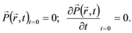
In this case, the general solution of Equation (22) consists of a particular solution (28) and two fundamental solutions of the homogeneous wave equation:

(32)

By taking into account initial conditions, we can reduce the solution (32), both for electron and nucleon, to the form:

(33)

The characteristic feature of the solution above is that the electrical polarization for both electron and proton, covers the entire infinite space and oscillates synchronously with the frequency ω_e,n;0.

The solution (33), however, contains a substantial disadvantage: such wave packet cannot move in space, it is a typical standing wave. Impossibility of motion is caused by the fact that the phase velocity of different harmonics v_f = ω_k / k changes from infinity to the light velocity c, whereas the group velocity v_g = ∂ω_k / ∂k changes from zero to c.

In a general case, the solution for the polarization for a wave packet moving with velocity should have a soliton form:

(34)

A similar property is natural for the solution of a onedimensional D’Alambert equation that fulfills the condition of deviation from a state of equilibrium for a flexible infinite string u(x,t) = u(x ± ct). A possibility of motion without changing the form is directly connected to a linear excitation spectrum in k-space ω_k = ck. For twoand three-dimensional cases, the solution of the D’Alambert equation substantially differs from the one-dimensional one. An excitation generated in some point starts propagating at velocity c in the form of concentrated circles for two-dimensional case, and in the form of concentrated spheres for the three-dimensional case. The propagation of radio waves strictly follows the three-dimensional D’Alambert equation, which proceeds from the Maxwell equations. Radio waves, however, are a multiquantum process. Nevertheless, a single quantum, while having wave properties, yet behaves like a particle. The thing is that a light quantum radiated by an excited atom at a distant star can cover million years without spreading dispersion. After colliding with a similar atom on the Earth, the light quantum transfers into a similar state of excitation. Therefore, there must be a solution of a soliton type for a light quantum in the form (34), which gives the origin of ray optics.

Analysis shows that it is impossible to obtain such a spectrum in a three-dimensional isotropic space for one order parameter. Following strictly the terminology, we should consider electromagnetic oscillations as coupled oscillations of a two-component order parameter in the form of an electric and magnetic polarization of vacuum.

Suppose a magnetic polarization with the same Hamiltonian, as that for the electric polarization (7) is possible to appear in vacuum:

(35)

We define a magnetic order parameter, as well as an electric polarization, through the sum of the elementary magnetic moments:

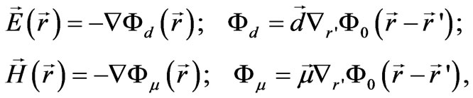
Practice shows that electric and magnetic dipole moments create, correspondingly, electric and magnetic fields, similar in configuration:

(36)

It follows that for a similar distribution of the electric and magnetic polarization, electric and magnetic fields will be similar as well. We can reduce expressions (36) to the form:

(37)

Here is the potential Coulomb function for a unit source. Under an arbitrary distribution of the electric and magnetic polarization, scalar potentials (37) acquire the form:

(38)

It follows that the sources of the electric field are the electric charges defined by the relation, whereas the sources of the magnetic field are the magnetic charges defined by the relation. As a result, the electric and magnetic fields meet the conditions:

Energy of the electric and magnetic fields turns up to be 137 times less than that of the electric and magnetic polarization, correspondingly. The configurations of the electric and magnetic fields are similar under the similar distribution of the electric and magnetic polarization. For example, if we create a homogeneous electric polarization in a full-sphere, then it causes generation of the depolarizing electric field inside the sphere; therefore, the depolarization coefficient for a sphere is equal to 1/3. The situation is the same with a spherical magnet:. Generation of the magnetic field also leads to the long-range Coulomb interaction between the normal oscillations: M_ex,M_ey,M_ez,M_nx, M_ny, M_nz.

We can define the electric current with the expression:

The continuity equation follows from here:

Now we show in what way the interaction between the electric and magnetic polarization provides the solution of the soliton type. We add the interaction energy of currents to the Hamiltonians (7) and (35) in the form:

(39)

From there we obtain the combined equations for a plane polarized electromagnetic wave:

(40)

By setting up the solutions in the form:

(41)

we can obtain the system of equations:

(42)

The compatibility condition for the Equations (42) leads to the equation:

This gives the spectrum of normal oscillations:

After that, the solutions for the electric and magnetic polarization transmitting with the light velocity reduce to the soliton form:

We proceed from the supposition that the electron radiates a light quantum; then from a wide range of possible solutions we should choose a solution compatible with the own field of the electron. Since the light quantum propagating along z-axis has a wave vector k_z, we can specify a Fourier-harmonic k_z from the scalar potential (27) which defines the field of the electron. In the cylindrical coordinate system, the Fourier-harmonic for the scalar potential becomes:

Here K₀ is the Macdonald function. We express the electric polarization along the x-axis as P_x = ∂Φ/∂x. Thus, for a plane-polarized wave compatible with the field of the electron and fulfilling the system of Equation (40), we obtain the solution for the electric polarization:

(43)

This solution is a quasi-one-dimensional infinite monochromatic wave propagating at the light velocity along the z-axis and interacting with the similar magnetic polarization M_y. In the transversal direction, the monochromatic wave (43) is localized with the dimension equal to the wavelength, since the Macdonald function at big values of argument approximately equals:

This precisely corresponds to the experiment, as it is impossible to localize a light ray more than the light wavelength.

Therefore, from the values, which we consider as fundamental e,ħ,c,m_e,m_p, we go over to the set of values, which characterize properties of physical vacuum under the additional condition: = c. In connection with this, we must change the concepts of mass and matter.

Wave equations can only be applied to the material medium having definite dynamic properties, so the idea of physical vacuum means that the entire infinite space is filled with a definite matter. The particles that we observe – electrons, protons, photons – these are excitations of vacuum in the form of wave packets, which are eigenfunctions of the united system of twelve equations. From the point of view of wave mechanics, we can characterize a wave packet with energy, momentum, angular momentum and oscillation amplitude; specifically for the electric polarization, we define the amplitude by the electric charge. For a multi-component order parameter, the form or symmetry of oscillations is important. In this connection, the concept of a particle mass does not have independent meaning. Researchers introduced the values of mass and charge, as well as Planck constant for particles, in different periods of time and so far, they have considered these values as independent ones. As we showed above, charge quantization and existence of Planck constant are the consequences of correlation effects related to discreteness of physical vacuum. Now it makes sense to study the concept of mass for a wave packet.

From practice we know that, if we describe the particle oscillation spectrum with the expression:

then the particle velocity is equal to the group velocity:

(44)

If we express the wave vector from (44) through the group velocity, we obtain the value of frequency in the form:

(45)

Multiplying terms of (45) by ħ, we come to the relativistic expression for the particle energy:

(46)

The expression for the particle mass m = E₀/c² follows from the latter Equation (46), the concept of mass being not necessary if we specify velocity in terms of light velocity.

The examples given below illustrate how to express some known values in terms of vacuum parameters:

De Broglie wavelength:

Here we have to consider k, the particle wave vector, as a quantum number independent of vacuum parameters.

Compton wavelength:

Classical radius of electron:

Bohr radius:

(47)

Bohr energy:

(48)

By making Bohr energy equal to photon energy,

we obtain quantum wavelength, which corresponds to Bohr energy

We can express Rydberg constant through vacuum parameters:

It follows from the above expressions that fine structure constant characterizes not only the fine structure of the hydrogen atomic spectrum but the entire lengths hierarchy of the quantum mechanics as well. It is easy to see that characteristic lengths form a geometrical progression:

All the lengths contain neither Planck constant, nor mass, nor charge of electron. In this connection, it makes sense to express the Schrödinger equation through the natural parameters of physical vacuum.

The Hamiltonian for the Schrödinger equation for a hydrogen atom looks like this:

In this expression, we take the fundamental constants ħ,m_e,0,e, which specify the characteristic parameters of a hydrogen atom (47-48), as independent; however, as we demonstrated above, none of these constants ought to be taken as a fundamental one.

We can write the Hamiltonian of the electron in the nuclear field of a hydrogen atom in a different form:

(49)

The Planck constant expressed through the electron charge reduces (49) to the form

(50)

Here, it is convenient to use the dimensionless length, the dimensionless wave vector and the dimensionless time. We express the energy in terms of the electron rest energy eg/r_c,e:

(51)

The particle velocity is equal to the group velocity of the wave packet and we express it in terms of light velocity. Approximate expressions correspond to the case of a low velocity k ≈ ν << 1 . We can regard the value k² in the approximate expression (51) as the eigenvalue of the Laplacian operator; then we may reduce (51) to the equation for the eigenfunction and the eigenvalue:

(52)

From (52) it follows that the Schrödinger equation only contains one dimensionless small parameter α of a physical vacuum susceptibility. The fundamental function Ψof a free electron in Cartesian coordinates is equal to; we express the eigenvalue by the equality:.

Now we find out the Bohr quantization conditions for a hydrogen atom. The circular motion of electron around an atomic nucleus is defined by the equality of centrifugal and centripetal forces:

. (53)

Bohr assumed a quantization of adiabatic invariants:

For the circular motion, the latter relation reduces to the form:

Externally, it looks as if a quantum of action existed, that provides quantization of a pulse moment. However, by taking into consideration the pulse p = ħk, we come to the cyclic boundary conditions for a wave vector:

It follows that Planck constant has nothing to do with forming the wave function. Since, we can add to Equation (53):

From where we can obtain the energy, radius and velocity at the stationary Bohr orbits:

That accurately corresponds to the relations (47,48).

Compton scattering, which we regard as one of the evidences proving existence of quantum of action, proceeds from the laws of conservation of energy and momentum for electron and quantum:

(54)

It follows from (54), that we can specify the wave vector of a scattered light by the relation:

(55)

Here θ is the angle between vectors and; besides, there is a length parameter where we take the values as the fundamental ones. However, by taking into consideration the fact, that relations (5) and (6) define the spectrum of a particle, we can reduce combined Equation (54) to the form:

It follows that the scattering characteristic is defined neither by the Planck constant nor by the electron mass, but by the space and frequency resonance for the wave packets; scattering being submitted to the same Formula (55) with the Compton length equal to the correlation radius.

Once in his days Planck supposed that radiation and absorption of light should proceed by quanta. Later this brilliant supposition was confirmed. After that, scientists had only to examine the properties of electron responsible for light radiation and absorption in a quantum way. Albert Einstein, however, considered something different. Since we can observe light quanta, then light is quantized due to existence of quantum of action; the question “Why?” being quite inappropriate here since physical mechanism for quantization of action just does not exist. We can only say that these are the properties of spaceime. We just substitute one senseless statement by anoher one. Nevertheless, proceeded from the fact that electron radiates and absorbs light per quanta, a planetary model of electron is suggested by itself. The electron rest energy equals to:. We can write quantum energy in a similar way:. Since the photon spin equals to, then, by representing it in the form of the orbital moment, we come to quite transparent cyclic conditions for the radius of photon orbit k_γ r_γ = 1. After that, the photon energy reduces to the form: ε_γ = eg/r_γ^. We can obtain such an energy as follows: use the solution for the electron polarization in the form (28), set it up into Hamiltonian (7) and integrate over space from infinity to the radius r_γ. Therefore, the nature of fields for photon and electron is the same. By radiating photon, an electron takes off some part of its polarization coat, the intrinsic energy of the electron being reduced.

3. Gravitaitional Optics

In the previous part we showed that all particles can be considered as excitations of physical vacuum; they are the solutions of the unified system of equations for coupled oscillations of the multicomponent order parameter. That is why we can be sure to a certain degree that all particles similarly contribute to the gravitational interaction, particle energy being the interaction parameter. Now we write down the standardized form of the Hamiltonian for a particle in the gravitational field caused by a massive body of mass m₁

(56)

We express the particle mass through energy ; after that the Hamiltonian (56) reduces to the form:

(57)

Here r_g is the gravitational radius which scales gravitational potential of a massive body. For an arbitrary potential, the Hamiltonian has the form:

In general case, particle energy is defined by the following expression:

(58)

In addition, particle velocity equals to

(59)

From the coordinate system (x,y,z,t) we proceed to a new time and, in Equation (58) – to a new momentum; then the particle velocity does not depend on the chosen scales of length and time, but becomes a dimensionless value expressed in terms of light velocity:

(60)

The second equation that defines the particle motion in the gravitational field looks like this:

(61)

By taking into account Equation (60), we can rewrite (61) as follows:

(62)

For low velocities we can substitute value by an approximate expression; after that Equation (62) reduces to that of Newton’s mechanics:

Based upon this equation, Albert Einstein affirmed that the inertial mass and the gravitating mass are equivalent. This statement, however, is incorrect. An accurate equation of motion (62) is transformed to:

(63)

It follows, that particle inertia depends on the direction of motion. It is interesting to note that the intrinsic (internal) energetic properties of a particle are lost in the equation of motion (63). This means that we can apply the obtained equation to any relatively compact object. It can be a planet, a satellite, an electron, a proton, a photon, a neutrino—all the same.

Bearing in mind (60), we reduce (61) as follows:

From the latter equation we obtain the integral of motion in two different forms:

(64)

Now we examine the motion in the Coulomb potential with the Hamiltonian (57). In a centrally symmetrical field motion develops in a plane crossing the centre of a massive body; therefore, we can re-write Equation (63) for the plane (x,y):

(65)

In the polar coordinate system Equation (65) becomes

(66)

The second equation in (66) can be integrated easily; after that we obtain the integral of motion corresponding to the angular momentum conservation law:

(67)

At the beginning, we consider a circular motion:. Then, the first equation of (66) leads to

(68)

This exactly coincides with the results of Kepler’s problem, the first space velocity on the orbit of radius r being equal to

(69)

Consequently, the first space velocity attains to the light velocity at r = r_g.

Further, we consider an arbitrary motion relative to a heavy centre. Let us assume that at time t = 0, a particle has coordinates (r = r₀, φ = 0), complete velocity v₀ and azimuth velocity. From the integrals of motion (64, 67) it follows:

(70)

From the system of Equation (70) we obtain the equation that combines φ and r:

(71)

Now proceed to a new variable 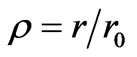and new parameters of the problem:

(72)

We examine the situation when the radial velocity at the starting point is zero. It follows that; after this, Equation (71) acquires the form

(73)

Here, the parameter δ defines a deviation from the circular motion in an orbit. We apply the Equation (73) to the Solar system. The gravitational radius of the Sun equals to 1.5 km. The radius of the terrestrial orbit is 1.5 10⁸ km, the radius of Mercury orbit is 0.5 10⁸ km, the radius of the solar sphere is 6. 96 10⁵ km. The parameter β in (73) is equal to for the Earth planet; to for the Mercury; and to for the Sun surface. It follows that the circular orbital velocity of the Earth is. In dimensional terms the circular velocity of the Earth equals to 10^-4c = 30 km/cek The Mercury moves in an elliptic orbit according to (73), where the value β << 1. Second order expansion in series of the exponent (73) leads to the equation

(74)

It enables to obtain the orbit path

(75)

We can find the complete revolution of the path from the condition:

Consequently, the angle gain over one revolution of the path is

.

The century displacement of the Mercury perigee means that while the Earth makes 100 revolutions around the Sun, the Mercury makes the number of revolutions equal to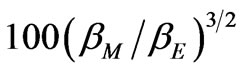. From here we obtain

(76)

The value is the eccentricity of the Mercury elliptic orbit.

From (75) we can obtain the condition when an elliptic orbit transforms into a parabolic path:

It follows that the second space velocity is a little less than that of Kepler’s problem and is equal to

(77)

Further, we consider the motion of a photon or a neutrino in a gravitational field. In this case, for the equation of motion (71), it is necessary to assume v₀ = v_φ0 = 1. Then, Equation (71) leads to

(78)

In order to calculate the complete angle of displacement for a light beam passing a gravitating mass, we move to a new variable and, as a result, we obtain:

(79)

Integral (79) is divergent at. It proceeds from the fact that at the gravitational radius a photon has a stationary orbit. For β << 1.

(80)

it follows that the deviation of a light beam moving, for example, along the Sun surface is. The only stationary orbit for a photon is that corresponds to the parameter. The slightest deviation from unit makes a photon either leave for infinity, or fall down to the centre. Figure 1 illustrates a photon getting off a stationary orbit.

Now we study a radial motion which we can determine from the integrals of motion (68). Under the given input conditions of the coordinate and velocity directed along the radius, and by using the integrals of motion (68), we obtain the energy of a photon moving away from the centre:

(81)

It follows that the photon crosses freely the gravitational radius and at the infinity the photon energy equals to:

(82)

The radial velocity of the photon remains constant;

The velocity of particles with non-zero mass is defined by the equation:

(83)

From (83) we can define the second space velocity:

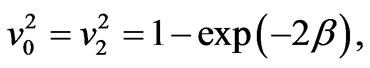(84)

it follows from (84) that at the initial velocity v₀ > v₂, any particle crosses freely the gravitational radius and leaves for infinity. Note that the first space velocity v₁ equals to. A circular orbit is steady under the condition that v₂ > v₁ from the equation

we define the boundary of stability for circular orbits. Circular orbits are only stable to small disturbances under the condition. This situation is described by the equation of motion (73) where we can consider the value of as a disturbance of a circular orbit. It follows from (73) that for any small value makes a particle leave for infinity along the path similar to that shown on Figure 1 (curve 1). Under the disturbance, a particle falls down to the centre and as well leaves for infinity along the curve similar to 2, 3 on Figure 1.

Since all bodies in the Solar system obey the same equation of motion (66), we can measure time in terms of any periodical process that occurs in the Solar system; for example, in terms of revolution of the Earth around the Sun. Further, since we can calculate the periods of revolution for any bodies beforehand, time in the entire Solar system runs similarly. Moreover, we extend the time over the entire visible part of the Universe; and we are quite right when we measure time in billions of years, whereas we measure distance in billions of light years.

Therefore, following Newton, we can repeat that a particle moves uniformly and straight until no force is applied. Following Galilee, we can say that under the same initial conditions in the gravitational field all particles move along the same paths. For example, under the same initial conditions an ultra relativistic proton moves in the same path as a photon does. However, Einstein’s statement that time runs differently in each lift does not have any physical meaning, since every electron covers the entire infinite space (33) and simultaneously interacts with all particles in the Universe.

4. Problems of Dark Matte

In the previous section we introduced the concept that it is the total particle energy which plays the key part in the gravitational interaction, but not the rest mass, as it is usually considered. This fact substantially changes the estimations of the matter quantity participating in the gravitational interaction. For example, the protons whose energy achieves 10²¹ eV in cosmic rays create a gravitational potential 10¹² times higher than that for protons on the Earth whose energy is 10⁹ eV. The situation is similar for neutrino. The mean energy of neutrino emitted by neutron beta decay is about 10⁶ eV; whereas zero energy of neutrino, which we usually take into account for gravitational interaction, is estimated by value of 10 eV. Consequently, neutrino contributes into the gravitational interaction 10⁵ times more. Photons having zero mass are not considered as carriers of the gravitational interaction at all. Deviation from the straight motion for a photon is caused by the Einstein deflection effect. This point of view contradicts elementary physics. The thing is that, if two bodies exist at positions and, and interact according to the law, then their momenta and follow the equations

(85)

Since

(86)

then, as a consequence of (85,86), follows the law of total momentum conservation:

(87)

Thus, the distortion of the trajectory for a photon passing e.g. the Sun shows(demonstrates) the variation of its momentum; it follows from the law of the total momentum conservation that the momentum of the Sun changes by the same amount. We can make an obvious conclusion: if a photon is attracted to a massive body, then the massive body is attracted to the photon to the same extent. Therefore, photons, like any other particles, participate in the gravitational interaction, interaction intensity being proportional to the proper intrinsic energy of the particle:.

The azimuth velocity of stars in galaxies is about 100-200 km/sec. That is why, the dark matter elements belonging to a certain galaxy at first sight may seem to have the same velocities. Hence, all relativistic particles, such as photons, neutrino, and cosmic rays, are beyond our consideration; as a result, practically none of the observed particles can create an additional gravitational field. In this connection an idea arises that there are heavy cold particles contributing only to the gravitational interaction; they are called dark matter.

However, a possible alternative point of view exists. First, we examine a simple example. A charged ion of a hydrogen atom creates a Coulomb potential where localized states for an electron are formed. Filling up one of the localized states makes the hydrogen atom electrically neutral, as the nuclear field is completely screened by an electron. On the other hand, if we insert a proton into a metal where there is a sea of free electrons, the localized state does not occur, but this time the nuclear field is screened by free electrons. The trajectory of each electron is distorted near the nucleus so much, that, as a result, electron density increases exactly to the same extent and it screens the nuclear field completely. A positive charge interacts with all free electrons of metal in a Coulomb way and attracts them.

Any heavy body attracts all free particles of a cosmic space by the gravitational interaction in a Coulomb way as well. Nevertheless, there is a significant difference between these two processes. Free electrons of metal are attracted to a positive charge, begin repulsive from each other, as a consequence, the electrical field of the positive charge is screened by electrons. The situation is quite opposite with the gravitational interaction. A massive body attracts particles from the surrounding space. Due to this attraction the total gravitational potential increases, thereby increasing the particle attraction even more. A positive feedback or antiscreening arises that can lead to the system instability. As an illustration, we examine the both situations: screening of an electrical field by free electrons in metal and antiscreening of a gravitational field by free particles (any) in cosmic space.

An external charge with harmonics placed into a metal creates a real charge defined as a sum of external and induced charges:

(88)

We can express the induced charge through the polarizability of electrons in metal.

Here; k_TF is a characteristic wave vector calculated using a Thomas – Fermi approximation [8]. As a result, we obtain

(89)

Here k_F is a Fermi momentum in metal. It follows from (89) that a Coulomb potential of a point charge q, for example, is transformed into a screened potential:

Now we consider a situation rather close to the gravitational interaction. Suppose, the entire space is filled up with neutral particles that have some homogeneous density and interact according to the law of gravitation. If any density fluctuation occurs in the space, then, owing to the gravitational interaction, all other particles begin to adjust to this density; there-after we can re-write the real density in the form:

(90)

On the analogy of a free electrons susceptibility, we imagine a gravitational susceptibility like this:. Here depends on the value of and on the distribution function of the particle velocity. Afterwards, the real density acquires the form:

This causes gravitational instability of the system relative to the long-wave density fluctuations. As fluctuations develop, slow particles, which compose a small part of an average density, are pulled out of the surrounding space and transformed into clusters of matter in form of stars and galaxies. Fast relativistic particles remain free and continue to participate in creating an additional gravitational field. We denote clusters of a cool matter in form of stars and galaxies having finite motion as. The remainder relativistic particles in form of cosmic rays, photons and neutrino create additional nonhomogeneous matter density due to the trajectory distortion. Here is the gravitational polarizability of the relativistic particles. Thus, the total density is equal to

Being on Earth, we have no possibility to scan the distribution of a total energy over the entire space. However, judging from the fact that the azimuth velocity of stars moving away from the centre of galaxy remains nearly constant, the total gravitational potential must have the form:

Here η is a dimensionless parameter, R_c– a gravitational size of a space belonging to a certain galaxy. Provided that the centrifugal and centripetal forces are equal

we come to the expression for the circular velocity:

At the star velocity being approximately equal to 200 km/sec we obtain the value. From the expression for the potential and with the aid of the Poisson equation we obtain the space distribution density of matter:

The space integral of density provides a value of mass inside a sphere of radius R:

For our Galaxy having the size of about R = 5·10⁴ light years and velocity of v = 200 km/sec we obtain M_i = 10⁴⁵ gr Mass of cool matter is estimated by value , therefore, mass of a relativistic matter is comparable with that of the cool one. Thus, as a result of the trajectory distortion for relativistic particles, an additional nonhomogeneous distribution of relativistic matter occurs and, consequently, an additional gravitational potential as well. That is why, there is no need to search for a mystical dark matter; relativistic energy is quite sufficient to create an additional gravitational field. Moreover, emission of radiation by stars and galaxies as well as supernova outburst lead to the constant growth of relativistic energy in space. So, observations of the azimuth stellar motion both in galaxies and galaxies in clusters point to the existence of an additional gravitational field. Since azimuth and radial motion follows from the general equation of motion, for example in form (63), the radial motion is submitted to the same additional gravitational attraction; for this reason, there is no dark energy to create antigravitation [9,10]. Thus, if red shift is related to recession of galaxies, then a contradiction arises, because galaxies have to scatter with acceleration but, judging from the azimuth motion, this is impossible.

It is more natural to consider atomic spectra of far stellar radiation to be time dependent as a consequence of time dependence of physical vacuum parameters. Since atomic levels are proportional to Bohr energy, and Bohr energy, in turn, is proportional to the rest energy of electron (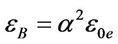) we can affirm that the electron mass increases with time; this means that vacuum parameters for the electron oscillation branch and decrease with time. The Hubble constant can be defined from the following expression:

(91)

The red shift indicates that the Hubble constant is a monotonically growing time function and at the present moment it equals to cek^-2.

Nowadays the Universe is in a metastable state, energy emission transitions occurring in two opposite directions. On one hand, nucleosynthesis of light nuclei—takes place, which is the source of stellar energy. On the other hand, nuclear disintegration of heavy nuclei (natural radioactivity) – occurs, as well with energy emission. From today’s point of view, nuclear fusion looks quite natural as there is a binding energy between nuclei; moreover, the binding energy on one nucleus increases with the growth of atomic number up to iron. Creation of heavier elements turns out to be less gainful; in this connection it is a surprise that heavy elements, up to uranium, exist on Earth. Nuclei of uranium are in metastable state. If we launched a piece of uranium towards the Sun, the uranium nuclei, under neutron bombardment, would decompose into lighter fragments. This means that uranium cannot occur on Sun. Deposits of uranium on Earth, however, prove that the Earth is an earlier formation than the Sun. Chemical composition of the Earth principally differs from that of the Sun. Sun consists of 75% hydrogen, 24% helium and a negligibly small amount of heavier elements, whereas Earth consists of 32% iron, 30% oxygen and a noticeable amount of heavier elements up to uranium. Heavy elements existing on Earth, as well as the red shift, point out to nonstationarity of physical vacuum parameters. Heavy elements could only occur on Earth when they were energetically gainful; variations of physical vacuum parameters led to the transition of heavy nuclei into a metastable state. A further evidence of nonstationarity of physical vacuum parameters is that not only stars, but also planets emit energy; moreover, volcanic activity, similar to that on the Earth, is still being observed on Jupiter satellites. It is known that the Jupiter emits twice as much energy as it receives from the Sun. We can express the Jupiter energy emission via the Hubble constant. From the law of conservation of energy it follows:

(92)

Here M_J c²– is Jupiter energy of erg, and L_J is the integral emission flux of erg/sec. By dividing both parts of (92) into Jupiter energy, and considering that the Jupiter only consists of hydrogen, we can reduce (92) to form

(93)

Here l_J is specific luminosity of the Jupiter equal to. Taking into consideration the definition of the Hubble constant (91), we can rewrite Equation (93) as follows:

(94)

All values at the right part of (94) are known, therefore,

So, the red shift shows that the rest energy of the electron is growing with time, whereas emission of radiation by planets indicates that the rest energy of the proton is decreasing; the total change of the energy for the electron and proton is so great, that it leads to planet heating and emission of radiation.

Since physical vacuum has existed eternally, the values, which characterize the vacuum, can only be of two types: either time independent constants, or oscillating functions. The fundamental values are general for both electron and nuclear modes seem to be thought as constant values; however, we have to consider as time dependent the values, which are characteristic either for an electron mode only by, or for a nuclear one—by. At the present moment electron and nuclear frequencies are moving towards each other.

Finally, we pay attention to one more mechanism of a gravitational instability. Not coincidentally, there has been some cause for concern so far, that microscopic black holes are possible to occur under the experimental research with Large Hadron Collider in CERN. The thing is that the gravitational attraction between particles grows with increasing particle energy, whereas, the electrical repulsion remains constant due to the law of conservation of charge. In this connection we examine two protons which are speeded up to a certain energy in an accelerator. We write down the Hamiltonian for two protons, taking into account an electrical and gravitational interaction:

Since masses of the particles are proportional to their energy m₁ = ε₁/c², m₂ = ε₂/c², then, under the following condition

the gravitational attraction turns out to exceed the electrical repulsion. Consequently, the gravitational collapse may occur when the particle energy amounts to

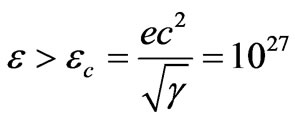eV.

Maximum particle energy in cosmic rays reaches 10²¹ eV. The value of energy expected at the accelerator in CERN is 7 ∙ 10¹⁵ eV that is eleven orders less than the critical value. That is why the microscopic black holes are impossible to appear in the accelerator. From the expression for the critical energy, we can define the specific wave vector and the corresponding de Broglie wave length:

It follows:

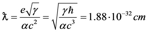
Planck introduced the specific length by reason of dimension:

.

It is easy to see that the specific length can be expressed via Planck length as follows:

Thus, the considerations above allow attaching a physical sense to the Planck length, which defines the most probable value for the lattice constant of physical vacuum; here k_c specifies the edge of the Brillouin zone in space, and– the width of the allowed energy region.

5. Conclusions

In presented paper we try to consider problems of the gravitational optics and dark matter developing from the crystal model for the vacuum. Thus, our model for vacuum is represented as a material medium in which dynamical properties of the crystal specify the spectrum of elementary particles . How it is follows from consideration it enables to describe both electromagnetic waves and spectrum of elementary particles from the unified point of view. We have obtained the combined equations for a multicomponent order parameter in the form of the electric and magnetic vacuum polarization, which defines the spectrum and symmetry of normal oscillations in the form of elementary particles. We have restored the fundamental parameters of physical vacuum, such as: a susceptibility for the electric and magnetic polarization (equal to the constant of fine structure), parameters of length and time for the electron and nuclear branches of the oscillations, correspondingly. We have shown that the charge quantization is directly connected to discreteness of vacuum consisting of particles with the interaction constant equal to the double charge of a Dirac monopole. Elementary particles are excitations of vacuum in a form of wave packets of a soliton type. We have obtained an exact equation of motion for a particle in a gravitational field. Energy defines both gravitational interaction and particle inertia, inertia being of an anisotropic value; that is why the statement, that the inertial and gravitational masses are equivalent, is not correct. We have examined the situation when galaxies are distributed over the entire infinite space according to the cosmological principle. In this case recession of galaxies is impossible; therefore, the red shift of radiation emitted by far galaxies must be interpreted as the blue time shift of atomic spectra. As a consequence, it follows that both rest energy and mass of electron are increasing now. Since physical vacuum exists eternally, vacuum parameters can be either constant or oscillating with time. These are time oscillations of and which have caused electron mass growth within recent 15 milliard years, inducing red shift; on the contrary, proton mass decreases, responsible for emission of radiation by planets.

REFERENCES

- F. Zwicky, “Die Rotverschiebung von extragalaktischen Nebeln,” Helvetica Physica Acta, Vol. 6, 1933, pp. 110- 127.
- K. C. Freeman, “On the Disk of Spiral and So Galaxies,” Astrophysical Journal, Vol. 160, 1970, pp. 811-830.
- J. A. Tyson, F. Valdes, J. F. Jarvis, and A. P. Mills, Jr., “Galaxy Mass Distribution from Gravitational Light Deflection,” Astrophysical Journal, Vol. 281, 1984, pp. L59- L62.
- A. G. Riess, A. V. Filippenko, P. Challis, A. Clocchiatti, A. Diercks, P. M. Garnavich, R. L. Gilliland, C. J. Hogan, J. Saurabh, R. P. Kirshner, B. Leibundgut, M. M. Phillips, D. Reiss, B. P. Schmidt, R. A. Schommer, R. C. Smith, J. Spyromilio, C. Stubbs, N. B. Suntzeff and J. Tonry, “Observational Evidence from Supernovae for an Accelerating Universe and a Cosmological Constant,” Astrophysical Journal, Vol. 116, No. 3, 1998, pp. 1009-1038.
- S. Perlmutter, G. Aldering, G. Goldhaber, R. A. Knop, P. Nugent, P. G. Castro, S. Deustua, S. Fabro, A. Goobar, Groom, I. M. Hook, A. G. Kim, M. Y. Kim, J. D. E. C. Lee, N. J. Nunes, R. Pain, C. R. Pennypacker and R. Quimby, “Measurements of {OMEGA} and {LAMBDA} from 42 High-Redshift Supernovae,” Astrophysical Journal, Vol. 517, No. 2, 1999, pp. 565-586.
- E. Q. Milne, “A Newtonian Expending Universe,” Quarterly Journal of Mathematics, Vol. 5, No. 1, 1934, pp. 64- 72.
- P. A. M. Dirac, “Quantised Singularities in the Electromagnetic Field,” Proceedings of the Royal Society of London A, Vol. 133, No. 821, 1931, pp. 60-72.
- D. Pines, “Elementary Excitations in Solid,” W.A. Benjamin, New-York, 1963.
- A. D. Chernin, “Dark Energy And Universal Antigravitaition,” Physics-Uspekhi, Vol. 51, No. 3, 2008, pp. 253- 282.
- V. N. Lukash and V. A. Rubakov, “Dark Energy: Myths and Reality,” Physics-Uspekh, Vol. 51, 2008, pp. 283- 290.