ABSTRACT

Tumor cells can evade immune surveillance by secreting immuno-suppressive factors such as transforming growth factor-beta (TGF-β) and also, Interlukin-10 (IL-10). In this paper the optimal control of mathematical model for aggressive tumor growth via a new and proper approach known as AVK method has been considered. Moreover, we have implemented a special treatment so-called small interfering RNA (siRNA) to reduce presence and effect of TGF-β in tumor cells and also we have added Interlukin-2 (IL-2) into our treatment model to minimize the population of tumor cells. Further research and experimentation with these combination therapies may provide an effective solution in addressing the immuno-suppressive effects of TGF-β. Finally, we analyze the optimal control and system optimality of these equations using numerical techniques.

1. Introduction

The concept of immunotherapy is based on the body’s natural defense system, which protects us against a variety of diseases. Although we are less aware of it, the immune system also works to aid our recovery from many illnesses. Immunotherapy falls into three main categories: Immune cell-stimulating cytokines, monoclonal antibodies, and vaccines. Cytokines are a number of small proteins that carry signals locally between cells, and thus have an effect on other cells [1]. Interleukin-2 (IL-2) is the main cytokine responsible for lymphocyte activation, growth and differentiation. IL-2 unlike classical chemotherapy does not kill tumor cells directly. Instead, IL-2 activates and stimulates the growth of immune cells, Natural Killer Cells (NK Cells) and most importantly T-Cells which are capable of destroying cancer cells directly [1]. Transforming growth factor-beta (TGF-b) is also one of the family cytokines, which are present in both healthy and tumor cells [2,3]. Although TGF-β promotes healthy cell growth and function, the production of TGF-b by tumor cells greatly challenges the immune system through the promotion of angiogenesis, enhancing tumor growth and metastasis [2]. In recent years several papers have begun to investigate the various aspects of the immune system response to cancer from a mathematical perspective. One of the first attempts to consider effects of immunotherapy was presented by Kirschner and Panetta. They study on the role of IL-2 adding with adoptive cellular immunotherapy (ACI) [4]. Sarkar and Banerjee, expressed the model which consist of three ordinary differential equations, tumor cells, hunting predator cells and resting predator cells [5]. Capputio et al. analyzed the interaction between NK cells, cells and effect of Interlukin- 21 (IL-21) in immunotherapy of tumor growth. They investigated effect of IL-21 on tumor cells. Then a year later they suggested optimal treatment of tumor cells via IL-21 [6]. In 2009 a mathematical models was presented by Jushi et al. They develop a new mathematical model of immunotherapy and cancer vaccination, focusing on the role of antigen presentation and co-stimulatory signaling pathways in cancer immunology [7]. Finally lets us to mention a recent paper by Arciero et al. which is presented a novel treatment strategy known as small interfering RNA (siRNA) therapy [8].Their model predicts conditions under which siRNA treatment can be successful in transformation of TGF-b producing tumors to either nonproducing or producing a small value of TGF-b tumors, that is to a non-immune evading state.

In this paper, we try to extend the model of aggressive tumors presented by Arciero et al. [8] and add IL-2 in their mathematical model to enhance ability of immune systems. We will implement optimal control theory for decreasing the population of tumors cell. Finally we desire to solve non-linear equations existing via a new and proper method named AVK.

2. Immunotherapy of Tumors siRNA

Through small interfering RNA (siRNA) treatment the initial delivery of double-stranded RNA (dsRNA) are taken into tumor cells (see Figure 1). Then the dsRNA is divided into 21 - 23 nucleotide-long segments known as siRNAs by enzyme Dicer. In that sense, enzyme Dicer target TGF-β mRNA once bound to the RNA-induced silencing complex (RISC) [5]. Complementary mRNA strands which is coded for TGF-β within tumor cells are determined by siRNA, subsequently, the RISC binds to and cleaves the mRNA to prevent production of TGF-β protein. Ultimately, siRNA treatment works to target the specific mRNA due to inhibiting TGF-β expression. Nevertheless, some drawbacks exist in this therapeutic strategy that may limit the effectiveness of it, such as the accessibility of siRNA target sites on TGF-β mRNA [9]. Moreover, cytokine therapy (e.g. IL-2 therapy) can be administered in combination with siRNA treatment, to not only inhibit the production and immuno-suppressive effects of TGF-β but also, increase ability of immune systems [2].

3. Aggressive Tumor Model

Aggressive tumor can produce TGF-β which is causing increased tumor growth from angiogenesis and the increased ability of the tumor to escape detection by the immune system due to immuno-suppressive properties. In [4] the mathematical model of passive tumors includeing effector cells, tumor cells and IL-2 are presented. In this paper we present a mathematical model for aggressive tumor where E(t) is effector cells as a immune system of body, T(t) is tumor cells, I(t) is IL-2, and S(t) is related to production of TGF-β as a immuno-suppressive factor [8].

(1)

(2)

(3)

(4)

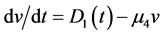
In Equation (1), effector cells are assumed to be informed of the tumor site in case the tumor cells are existed. The parameter c in the first term of Equation (1), measures the ability of the immune system to recognize tumor cells which is known as antigenicty of the tumor. Inhibitory parameter γ is a factor to show production of

TGF-β which is lead to decrease antigen expression [2]. The second term represents the mortality rate of effector cells. The third term, Michaelis-Menten forms of components, presents effector cell proliferation due to presence of the cytokine IL-2 that can decrease when the cytokine TGF-β is produced. Where p₁ is the maximum rate of effector cell, g₁ and q₂ are half-saturation constants, and q₁ is the maximum rate of anti-proliferative effect of TGF-β.

Equation (2) is related to the growth of the tumor cells. The first term represents logistic growth of tumor cells where r is intrinsic growth rate and K is carrying capacity of tumor in the absence of effector cells and TGF-β (or every simulated factor). The second term describes the reduction of the tumor population depends on immune clearance. The interaction between immune response and tumor cells is measured by parameter a [4]. The third term in Equation (2) accounts for the increased growth of tumor cells because of TGF-β production. In fact, TGF-β is a factor helps tumor cells to exceed their size. This term is a form of Michaelis-Menten which indicates a limited response of tumor cells to a growth-stimulatory cytokine like TGF-β. Also, p₂ is the maximum rate of increased proliferation and g₃ is the half-saturation constant.

In Equation (3) the kinetics of IL-2 is explained. The first term shows IL-2 production with a maximum rate of p₃ in the presence of effector cells stimulated and with a half-saturation constant g₄ without considering TGF-β as a limited cause. In addition, parameter α measured the inhibition of IL-2 production in presence of TGF-β in an uncompetitive manner. In last term, the decay rate of IL- 2 is represented by μ₂.

Equation (4) describes the rate of change in producing suppressor cytokine, TGF-β with p₄ as the maximum rate of TGF-β production and t_c as the critical tumor cell population in which the switch occurs. Furthermore, μ₃ represented the decay rate of TGF-β [8]. For more details about parameters which are used in these equations we can say that where it is possible, these parameters are taken from the medical literature and articles, and when there are unavailable experimental data for some parameters, we consider our goal to quantify the parameters influence on the model behavior. Table 1 lists the baseline values of the model parameters used in the numerical simulations. Briefly, values for the parameters are used without considering last equation. It means that we assume. The equations are nondimensionalized as follows [8]:

(5)

Then, without considering over-bar notation for convenience, the system of tumor growth in the absence of treatment is represented as below [8]:

(6)

(7)

(8)

(9)

With initial conditions

In this section, we describe the case in which tumors become aggressive and interfere the body’s immune response when TGF-β is produced, tumor mass has enough potential to grow near its carrying capacity and this situation can occur for all tumors at some p₄ value, regardless of the level of antigenicity. The three figures illustrate the different results when increasing the rate of TGF-β production (p₄) for various values of antigenicity (c). In Figure 2, the value of c and p₄ are very small (c = 1 × 10^–10). Therefore, tumor cannot be detected by the immune system. This result in rapid tumor growth quickly approaches its carrying capacity. Figure 3 presents an intermediate value of c (c = 0.002) and two different value of p₄, p₄ = 0 and 0.1, it clearly show that the more value of p₄, the greater tumor growth. Also, uncontrolled tumor growth is suppressed. Finally, Figure 4 represents the lowest value of c (c = 0.0035) at which the

immune system has ability to control the tumor population. Tumor’s behavior has damped oscillations and shows downward trend. This manner sometimes is described as dormant. However, if p₄ increases, the immune system is no longer successful in defeating the tumor, and large tumor mass again characterizes the tumor behavior near carrying capacity.

4. Optimal Treatment of Tumors Using siRNA and IL-2

In this section we have provided one of the mathematical models of aggressive tumor growth that implements siRNA treatment to suppress TGF-β production. In this paper, we incorporate IL-2 by defining a controller to the model. While not yielding persistent dormancy, siRNA offers a treatment technique that counteracts the devastating effects of TGF-β, such as IL-2 inhibition and increased tumor growth. Variable of u(t) is percentage of applying drug during immunotherapy that we expected to achieve the existing status of patient to desirable defining status. Therefore, we define a mathematical model Equations (14)- (18), including siRNA to suppress effects of TGF-β at tumor cells and also, IL-2 to enhance effects of immune system. Notice that the first three equations correspond to Equations (1), (2) and (3). Moreover, Equation (13) is modified version of Equation (4) that concentrates on cytokine TGF-β [8].

(10)

(11)

(12)

(13)

(14)

In the first term of Equation (13), the production of TGF-β due to effects of siRNA is inhibited; indeed, siRNA is bound to target TGF-β mRNA. Variable A represents total strands of siRNA, free and bound strands, and parameter f shows the proportion of variable A which is bound. Thus, the bound siRNA strands are described by fA, and k_i measures inhibition rate of siRNA as a suppressive factor.

Equation (14) represents the injection and degradation of the siRNA. D₁ describes a continuous infusion dose of siRNAs as a function of time. So, D₁(t) = D₀ ≡ constant. In fact, D₀ is the injected dose. The second term, μ_4, represents the decay of the free siRNA strands based on their half life which is estimated of 0.66 days⁻¹ [10]. Also, in many vitro studies siRNA treatment have determined with an initial dose of 2 × 10⁹ pg/ml of siRNA [11]; therefore, we take D₀ = 5 × 10¹⁰ pg/ml as a comparable dose for an in vivo system. u(t) is a control function that explains percentage of using IL-2 and in this paper we recognize it as a continuous step function of time for each t relating to treatment period

If u(t) = 1 means maximum percentage of immunotherapy and u(t) = 0 is not using immunotherapy. The main object of u(t) is to improve the existing status of patient to defined desirable status

Firstly, the equations are nominated in nondimensional form. The scaling used is the same as in Equation (5) with the following additions:

(15)

Then, without considering the over-bar notation for convenience, the system describing tumor evasion of immune surveillance in the presence of siRNA treatment may be written as follows:

(16)

(17)

(18)

(19)

(20)

We can attain v(t) by solving Equation (20) according to value of its parameters (and) and then put it in Equation (19). Consequently, v(t) ≡ constant.

Often controllable problems have large dimensions and analyzing them is difficult so we try to estimate a control problem with linear programming then explain it via numerical results. In this method we first estimate our problem with calculus of variations then convert it with a linear programming problem. If the optimal answer of linear programming problem is zero or near zero, we can conduct system from one condition to another. Moreover answer of linear programming problem can provide proper estimation and desirable control of system. Attending to this subject, we can apply discriminating method for nonlinear systems, therefore in this paper we estimate mathematical model of tumor growths via AVK method [12] to nonlinear programming problem afterwards we can solve the nonlinear programming problem by LINGO software. We can approach exact answer of differential equation systems and achieve accuracy estimation by increasing the number of division points in range [a, b]. 

5. Objective Function and Multi Objective Optimal Control

In this paper, we use control rule of u(t) for decreasing tumor size via mathematical model, tumor size is decreased, and the prescribed dose is determined for the patient simultaneously. Therefore we intend to minimize multi objective optimization (Equation (21)) attentive to and weights w₁ = 0.8 and ww₂ = 0.2, so in this case we consider significance of minimizing tumor cells more than dose of prescription IL-2. Purpose of introducing this objective function is to decrease tumor cell population and amount of TGF-b by using external drug source whereas effector cells and IL-2 is sufficiently increased on round of treatment.

(21)

6. AVK Method

Definition 1: We focus on following nonlinear problems with uncertain parameter (NPUP)  

(22)

X and U are compact subsets and must be chosen as the system reaches from initial state x(t₀) = x_a to final state x(t_f) = x_b.

Definition 2: First, consider nonlinear system (22), we define following functional that is called the total error functional. Let

(23)

Where is a continuous functional.

Definition 3: The solution of uncertainty problem can track the desired curve x_d(t), if we consider a multi objective functional as

(24)

Definition 4: If t has D known distributed function similar to g(t), we may define new functional:

(25)

Theorem 1: If h is a nonlinear continuous function on and non-negative , then the necessary and sufficient condition for is h º 0 on.

Theorem 2: Necessary and sufficient condition for a nonlinear function to be concluded a NPUP (22), with initial condition x(t₀) and final state x(t_f) is to satisfy the following relation in problem (23):

Note: Without loss of generality, we may assume t₀ = 0 and t_f = 1.

Note: We can assume h(t) is a non-negative piecewise continuous functional in [0, 1] instead of non-negative continuous condition in [0, 1] and for h = 0 we may assume h(t) = 0, almost everywhere in [0, 1]

In AVK method, the following problem is defined in calculus of variations:

(26)

Where or all uncertain values, g(t) is a distribution function. We assume the optimal solution of problem (26) is x*(t), u*(t), the state and the control functions, respectively. According to Theorems 1 and 2:

(27)

Then in general, for solving NPUP (1) we can solve the minimization problem (26) by Theorems 1 and 2. Thus the optimal solution of problem (22) is x^*(t), u^*(t) from optimization problem (26).

We have in equivalent problem (26) so that D takes all values between [a₁, a₂]. Then divide the interval [a₁, a₂] is divided by n equal part. Let

Where k = 0, 1, ∙∙∙, n, and. We define non-consistent differential equation system:

(28)

We are looking for the best solution x^*(t), u^*(t) for the non-consistent differential equation system (28) where all discrete values of D are included. The best solution for the optimization problem (26) is minimizing the total error of above system, i.e. total error in L₁ space is minimized as follows:

(29)

Now, we will solve problem (29) approximately. We partition the interval to m equal subintervals (cells), where m is arbitrary fixed positive integer and then problem (29) yields to

For summarize, the initial value and final value are neglected. Let for the first derivative we have Suppose , thus the approximate value achieves to the best value for derivation at the time t. Hence dt or sampling time is very important, and must be chosen small, so the number of partitions is great. This is a tradeoff between sampling time and speed of problem solving. Also, we use L₁ norm as follows:

(30)

Remark: As we know, an approximate value of integral is (b-a). K(c), where c is any point such as. So, applying above remark, and assume c is an ending point in any subinterval, minimization problem (29) is formed as Equation (31) according to Equation (30).

(31)

where the unknown parameters are defined as below:

Thus t₀ = 0, t_m = 1, also, and Also assume:

Thus, we simplify obtained discretized problem (31) in the form

(32)

As a whole, problem (32) is a NLP problem and we may obtain its solution by many packages such as Lingo, Matlab, Gino, etc. Finally, by obtaining the solution of problem (32), we recognize the value of unknown admissible pair state and control function at points. We can construct the optimal solution for NPUP (22) by two piecewise functions Theorem 2 will show existence of the optimal solution for the NPUP (22) [12].

7. Simulation

After using AVK method for discrete equations, we will achieve a control problem (i.e. problem 32) by synthesizing objective function (21) with initial and final condition. Supposing the reason of aggressive tumor growth is inadequacy or inability of patient’s immune system that is caused to create tumor and finally death. We use one of the immunotherapies so-called cytokines IL-2 in order to improve immune system. The initial and final conditions are taken from clinical experiences. Considering T = 10000 (normalization round of treatment), n = 20 (number of divisions) and weights w₁ = 0.8 and w₂ = 0.2 to prove the effect of drug control on improving immune system. We can observe population of tumor cells and also external drug source control with optimal answer. In both Figure 5 and Figure 6, c = 0.002 and p₄ = 0.5. In general, we have tried to minimize population of tumor cells by adding objective function and an external drug source (injecting IL-2 cytokine parallel to siRNA treatment) under control. In Figure 2, the maximum number of tumor cells was shown about 10⁴ cells before treatment. Whereas, In Figure 5, the final number of tumor cells is about 10³ cells after using treatment (i.e. siRNA and IL-2) which means that we could manage to overcome 90% of tumor cells. Note that there is no situation in which tumor could be cleared by the body [4] so this is an acceptable result. If the amount of drug used at the end of treatment is paused, tumor cells start to grow again, so using drug has to be continued forever. Figure 6 shows percentage of using IL-2 as a drug to minimize number of tumor cells during a 1000-day period which indicates that how much drug is needed for each period.

8. Conclusion

The aim of this paper was to exhibit a new and proper approach, known as AVK method, which could solve the nonlinear equations without changing its structure. The fairly proper efficiency of this suggested method was shown by numerical results. As was described, siRNA treatment inhibits the production and immuno-suppressive effects of TGF-β by targeting the specific mRNA sequence which leads to its synthesis. Furthermore, adding IL-2 in to the model could result in controlling tumor by enhancing an immune response. The mathematical model of aggressive tumor was extended to include therapeutic strategy using siRNA and IL-2.  

9. Suggestion

An extension along this line of work will be to examine the effect of other cytokines such as IL-10, IL-12 and interferon-g, which are involved in the cellular dynamics of the immune system response to tumor invasion and how these cytokines affect the dynamics of the system. For future study, the addition of each cytokine above with other treatments such as chemotherapy and radiotherapy into our treatment model could result in actual tumor clearance.

REFERENCES

- A. K. Abbas, A. H. Lichtman and J. S. Pober, “Cellular and Molecular Immunology,” Elsevier, Amsterdam, 2007.
- K. E. de Visser and W. M. Kast, “Effects of TGF-β on the Immune System: Implications for Cancer Immunotherapy,” Leukemia, Vol. 13, No. 8, 1999, pp. 1188-1199. doi:10.1038/sj.leu.2401477
- M. A. Nash, G. Ferrandina, M. Gordinier, A. Loercher, and R. S. Freedman, “The role of cytokines in both the normal and Malignant Ovary,” Endocrine-Related Cancer, Vol. 6, No. 1, pp. 93-107.
- D. Kirschner and J. C. Panetta, “Modeling immunotherapy of the Tumor—Immune Interaction,” Journal of Mathematical Biology, vol. 37, No. 3, 1998, pp. 235-252. doi:10.1007/s002850050127
- R. R. Sarkar and S. Banerjee, “Cancer self remission and Tumor Stability: A Stochastic Approach,” Mathematical Biosciences, Vol. 196, No. 1, 2005, pp. 65-81. doi:10.1016/j.mbs.2005.04.001
- B. Joshi, X. Wang, S. Banerjee, H. Tian, A. Matzavinos and M. A. Chaplain, “On immunotherapies and Cancer Vaccination Protocols: A Mathematical Modelling Approach,” Journal of Theoretical Biology, Vol. 259, No. 4, 2009, pp. 820-827
- S. M. Mousavi1, M. M. Gouya, R. Ramazani, M. Davanlou, N. Hajsadeghi and Z. Seddighi, “Cancer incidence and mortality in Iran,” Annals of Oncology, Vol. 20, No. 3, pp. 556-563. doi:10.1093/annonc/mdn642
- J. C. Arciero, T. L. Jackson and D. E. Kirschner, “A Mathematical Model of Tumor-Immune Evasion and siRNA Treatment,” Discrete and Continuous Dynamical Systems, Vol. 4, No. 1, 2004, pp. 39-58. doi:10.3934/dcdsb.2004.4.39
- T. Holen, M. Amarzguioui, M. T. Wiiger, E. Babaie and H. Prydz, “Positional effects of Short Interfering RNAs targeting the Human Coagulation Trigger Tissue Factor,” Nucleic Acids Research, Vol. 30, No. 8, 2002, pp. 1757- 1766. doi:10.1093/nar/30.8.1757
- S. M. Elbashir, J. Harborth, W. Lendeckel, A. Yalcin, K. Weber and T. Tuschl, “Duplexes of 21-nucleotide RNAs mediate RNA interference in Cultured Mammalian Cells,” Nature, Vol. 411, No. 6836, 2001, pp. 494-49. doi:10.1038/35078107
- F. Wianny and M. Zernicka-Goetz, “Specific interference with Gene Function by doublestranded RNA in Early Mouse Development,” Nature Cell Biology, Vol. 2, No. 2, 2000, pp. 70-75. doi:10.1038/35000016
- K. P. Badakhshan, A. V. Kamyad and A. Azemi, “Using AVK Method to Solve Nonlinear Problems with Uncertain Parameters,” Applied Mathematics and Computation, Vol. 189, No. 1, 2007, pp. 27-34. doi:10.1016/j.amc.2006.11.172