ABSTRACT

The present study illustrates a series method for the solutions of one dimensional wave equation together with non-classical dynamic boundary conditions. Matheu-Hill form, a differential equation with polynomial form and Laguerre differential equation form dynamic boundary conditions were taken into consideration. Series methods were given in order for the solutions of wave equation together with these dynamic boundary conditions along with semi-infinite axis of the spatial coordinate. Wave profiles were obtained by means of wave solutions of the wave equation given by d’Alembert.

1. Introduction

One dimensional motions of many number of physical elements are governed by a partial differential equation, called wave equation. In order to model wave motion of a one dimensional physical element, it is required to have additional information besides just the wave equation. These compatibility conditions are called boundary conditions and initial conditions. The Fourier method, or separation of variables method is widely utilized to attain solution forms of the wave equation together with classical dynamic boundary conditions. Fourier and Laplace transform methods are also useful mathematical tools to derive the solutions of the wave equation together with the classical boundary conditions along the finite, infinite and semi-infinite range of the spatial coordinate. There is another approach dating back the eighteenth century which is known as d’Alembert solution. In order to write explicit form solutions, by means of changing the coordinates, this method transforms wave equation into canonical form [1-3].

Oscillation of some one-dimensional elements may result in a boundary value problem including Matheu-Hill differential equation form non-classical dynamic boundary conditions [4,5]. There are not any research articles that have discussed the one-dimensional wave equation together with non-classical dynamic boundary conditions in literature. In this study, we were concerned with the derivation of a series solution of the wave equation together with Matheu-Hill differential equation form, variable coefficient differential equation form and Laguerre differential equation form boundary conditions, along with the semi-infinite axis of the spatial coordinate. In order to avoid theoretical difficulties, we did not impose any initial conditions on these boundary value problems. We did not examine the stability of Matheu-Hill differential equation form boundary condition. Such an analysis requires Floquet Theory based further investigation.

2. Matheu-Hill Form Dynamic Boundary Conditions

d’Alembert solution of one dimensional wave equation involves two traveling waves, which are called backward and forward waves, respectively. The profile of the wave motion at a fixed time t is the sum of these backward and forward waves. In this section we derived a series solution for one dimensional wave equation together with Matheu-Hill differential equation form boundary condition along semi-infinite axis by using d’Alembert’s wave form solutions.

A differential equation, , where are constants, dots denote derivative with respect to time t, is known as Matheu-Hill equation, which is of great importance in the study of dynamic systems. Now, we will consider this differential equation as a boundary condition together with the wave equation. Let us regard one dimensional wave equation along semi-infinite positive axis of spatial coordinate x and impose MatheuHill equation as a boundary condition at. Then, we can write the corresponding boundary value problem as,

(1a)

(1b)

where dots and prime denote partial derivatives with respect to time t and spatial coordinate x, respectively. Note that the last term in Equation (1b) is the connection term between the equation and the boundary condition. The general solution of the wave equation is the sum of backward and forward wave form solutions, , i.e. 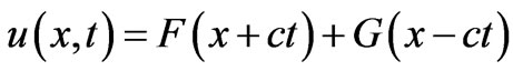. Hence, it can be expressed as Taylor series expension of summation of two variable, , and solutions can be sought in power series of backward and forward wave form solutions separately. Matheu-Hill equation form boundary condition (1b) has no singular points. Then, one can seek a power series representation of backward wave (or forward) for the solution of the boundary value problem (1) as,

(2)

Note that we are not concerned with the Floquet solutions, i.e. form stable and unstable solutions of the boundary value problem (1). For the sake of simplicity and further discussion, let us choose the physical constants as. If one expends the harmonic coefficient of the boundary condition (1b) as and then inserts solution form (2) into boundary condition (1b), one obtains,

(3)

If one combines summations and computes a few terms from Equation (3), one can write backward wave form solution as follows,

(4)

Figure 1 shows two linearly independent parts of backward wave profile,

for given arbitrary constants, in the interval.

3. Satisfying a Non-Classical Dynamic and a Simple Geometric Boundary Condition Simultaneously, Convoluted Odd Function

Let us now consider Matheu-Hill form boundary condition at and a simple geometric boundary condition at, together with the wave equation. In that case, the wave form solutions can be shifted with a constant lenght to the point. However the solution of the problem remains in similar form. We aim at deriving traveling wave solutions satisfying both wave equation and these two boundary conditions simultaneously.

For this purpose, let us select second (or first) independent profile and form the negative symetric of the wave profile with respect to the point and generate an extended odd function wave profile. Now, if the left part profile is moved to the right with the velocity c and the right part profile to the left with the velocity c, then two boundary conditions could be satisfied simultaneously (Figure 2). However, this solution satisfies two boundary conditions only with the period of time. Therefore it is not an exact solution. In order to

overcome this complex problem, let us define a convoluted piecewise continuous odd function generated from the wave form solutions as follows.

Definition. Let be a continuous function in the positive real axis x. Let be partitioned function of in the intervals .

A convoluted piecewise continuous odd function is

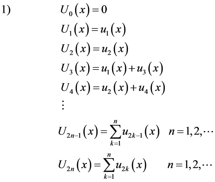
2)        

Now, if the left part of the is moved to the right and the right part to the left with the velocity c, two boundary conditions are satisfied simultaneously.

4. Polynomial Coefficient Form and Laguerre Form Dynamic Boundary Conditions

In this section, we investigated series solutions of the wave equation together with a variable coefficient form and Laguerre form dynamic boundary condition. Let us consider one dimensional wave equation along semi-infinite positive axis of spatial coordinate x and impose a polynomial coefficient form equation as a dynamic boundary condition at, as follows,

(5)

Note that dynamic boundary condition (5) has a singular point at. One can seek a Frobenius series representation of backward wave (or forward) for a solution of the boundary condition (5) as,

(6)

For the sake of simplicity and further discussion again, let us choose the physical constants as . If one inserts the series solution (6) into boundary condition (5), shifts indices and combines summations, then one obtains,

(7)

From Equation (7), one obtains the indicial roots as and writes two recurrence relations as,

(8)

If one uses the properties of factorial in the Equation (8) then one can write the backward wave form of the series solution (6) as follows,

(9)

where and are arbitrary constants.

Figure 3 shows two linearly independent parts of backward wave profile,

for given arbitrary constants , in the interval.

Let us now consider one dimensional wave equation along semi-infinite positive axis of spatial coordinate x and impose Laguerre form dynamic equation as a boundary condition at. The boundary condition can be written as follows,

(10)

Actually, Laguerre’s differential equation is a reduced form of radial form of Schrödinger’s equation. Hence, it states a spatial coordinate dependent differential equation. However, we imposed this equation as a dynamic boundary condition on the wave equation, because it seemed appealing and raised motivation on us. Note that Laguerre form boundary condition (10) has a singular point at. Then one can seek a Frobenius series representation of backward wave (or forward) for a solution of the boundary condition (10) as,

(11)

For the sake of simplicity again, let us choose the physical constants as. If one inserts the series solution (11) into boundary condition (10), shifts indices and combines summations, then one obtains,

(12)

From Equation (12), one obtains the indicial roots as and can write two equivalent recurrence relations as,

(13)

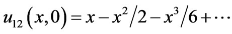
If one uses the properties of factorial in the Equation (13) then one can write the first independent part of backward wave form of the series solution (11) as a polynomial.

Since the roots of the indicial equation differ by a positive integer, there exists another solution which may contain a logarithm term,

5. Conclusions

It can be concluded that the wave form solutions may be a useful tool for the solution of one dimensional wave equation together with Matheu-Hill form, differential equation with polynomial coefficient form and Laguerre form non-classical dynamic boundary conditions. In this study, initial displacement and initial velocity conditions were not taken into consideration. The stability of the solutions, in the case of Matheu-Hill form boundary conditions, are not examined. Finaly, the solution method presented in this study does not cover the Fourier Method, so is not applicable for classical boundary conditions and boundary value problems.

REFERENCES

- P. V. O’Neil, “Advanced Engineering Mathematics,” Thomsons, 2003.
- L. A. Pipes and L. R. Harvill, “Applied Mathematics for Engineers and Physicist,” McGraw-Hill, Boston, 1970.
- K. F. Riley, M. P. Hobson and S. J. Bence, “Mathematical Methods for Physics and Engineering,” Cambridge University Press, Cambridge, 2006.
- K. Koser, “Torsional Vibrations of Drive Shafts of Machines,” Ph.D Thesis, Istanbul Technical University, Istanbul, 1993.
- K. Koser and F. Pasin, “Continuous Modelling of the Torsional Vibrations of the Drive Shaft of Mechanism,” Journal of Sound and Vibration, Vol. 188, No. 1, 1995, pp 17-24. doi:10.1006/jsvi.1995.0575