American Journal of Climate Change
Vol.05 No.02(2016), Article ID:67596,27 pages
10.4236/ajcc.2016.52019
A High-Resolution Modeling Strategy to Assess Impacts of Climate Change for Mesoamerica and the Caribbean
Robert Oglesby1, Clinton Rowe1, Alfred Grunwaldt2, Ines Ferreira2, Franklyn Ruiz3, Jayaka Campbell4, Luis Alvarado5, Francisco Argenal6, Berta Olmedo7, Alejandro del Castillo8, Pilar Lopez9, Edwards Matos6, Yosef Nava10, Carlos Perez11, Joel Perez8
1Department of Earth and Atmospheric Sciences, University of Nebraska, Lincoln, NE, USA
2Climate Change and Sustainability Division, Inter-American Development Bank, Washington DC, USA
3Instituto de Hidrología, Meteorología y Estudios Ambientales de Colombia, Bogota, Colombia
4University of the West Indies, Kingston, Jamaica
5Instituto Meteorológico Nacional Costa Rica, San Jose, Costa Rica
6Servicio Meteorológico Nacional de Honduras Dirección General de Aeronáutica Civil, Tegucigalpa, Honduras
7Empresa de Transmisión Eléctrica Panameña, Ciudad de Panamá, Panamá
8Water Center for the Humid Tropics of Latin America and the Caribbean (CATHALAC), Ciudad de Panamá, Panamá
9Unidad de Análisis Meteorológico, Empresa de Transmisión Eléctrica Panameña, Ciudad de Panamá, Panamá
10Instituto Nacional de Ecología y Cambio Climático, Mexico City, Mexico
11National Weather Service, MARN, San Salvador, El Salvador

Copyright © 2016 by authors and Scientific Research Publishing Inc.
This work is licensed under the Creative Commons Attribution International License (CC BY).
http://creativecommons.org/licenses/by/4.0/


Received 3 February 2016; accepted 17 June 2016; published 22 June 2016
ABSTRACT
Mesoamerica and the Caribbean are low-latitude regions at risk for the effects of climate change. Global climate models provide large-scale assessment of climate drivers, but, at a horizontal resolution of 100 km, cannot resolve the effects of topography and land use as they impact the local temperature and precipitation that are keys to climate impacts. We developed a robust dynamical downscaling strategy that used the WRF regional climate model to downscale at 4 - 12 km resolution GCM results. Model verification demonstrates the need for such resolution of topography in order to properly simulate temperatures. Precipitation is more difficult to evaluate, being highly variable in time and space. Overall, a 36 km resolution is inadequate; 12 km appears reasonable, especially in regions of low topography, but the 4 km resolution provides the best match with observations. This represents a tradeoff between model resolution and the computational effort needed to make simulations. A key goal is to provide climate change specialists in each country with the information they need to evaluate possible future climate change impacts.
Keywords:
Regional Climate Models, Dynamical Downscaling Strategy, Mesoamerica and Caribbean Climate Change

1. Introduction
One of the key gaps in the Intergovernmental Panel on Climate Change (IPCC) global reports, from the First through the Fifth Assessment, is the dearth of literature that exists for climate related studies for the small island states of the Caribbean, as well as Mexico, the isthmus nations of Central America and Colombia (collectively known as Mesoamerica and the Caribbean, or MAC). This area represents one of the regions with the largest global vulnerability to the impacts of climate change, not just because of their socio-economic condition but also because of their small size and extremely large coastal populations [1] - [6] . Indeed, the countries of MAC are already suffering the effects of climate change and their limited capacity to adapt, a product of its socio-economic context, makes them highly vulnerable.
While useful in projecting large-scale changes and effects, the coarse horizontal resolution of the CMIP5 global models used for the IPCC Assessment Report 5 (AR5) simulations (approximately 100 km) limits their usefulness when projecting changes at the regional or local scale. At these resolutions, GCMs can only adequately simulate basic large-scale features of climate. As stressed by IPCC, results at this global scale are useful for indicating the general nature and large-scale patterns of climate change, but not very robust at the important local or regional scales of approximately 10 km or less. This is for two reasons: 1) GCMs can only explicitly resolve physical processes operating over several hundred kilometers or larger, with smaller scale processes necessarily parameterized in terms of the large-scale ones; and 2) spatial surface heterogeneities, especially over land, can be very large and occur on small spatial scales. Examples of these heterogeneities include regions of complex topography or with heterogeneous land use patterns.
For MAC, several regional climate modeling studies have been conducted in an attempt to fill this void. For studies covering a majority of the MAC region, the simulations have been done using 50 km resolution. This resolutions appear adequate to provide some improvement over GCMs of regional circulation features such as the Caribbean Low-Level Jet (CLLJ), especially over open water [7] , but fail to adequately resolve near-surface variations associated with the complex terrain and micro-scale climate over land [8] [9] . Moreover, some seasonal features, especially during JJA and including the Mid-Summer Drought (MSD), remain poorly represented. In contrast, using a different RCM, Diro et al. [10] found the MSD well resolved but the CLLJ underestimated. Karmalkar et al. [11] also found some improvement due to better resolution of topography, but also found considerable precipitation biases―in magnitude, spatial distribution, and seasonal timing―when employing this model resolution.
Several studies have used somewhat higher resolution regional models, but for only a portion of the MAC [9] [12] - [14] and only at resolutions of 20 or 25 km, except for the Colombian Andes at 4 km [14] . In general, these studies found improved representation of temperature and precipitation patterns in the respective domains but not necessarily improvement in precipitation bias. In addition, small-scale circulation features such as sea breezes―at least over the larger islands―could begin to be resolved.
It is clear that previous modeling efforts have failed to properly capture the high resolution, local effects on climate due to topography and the nature of the land surface. But just what spatial resolution is necessary? And what modeling strategy is best suited to achieving this? How can this information best be provided to those experts who need it in the individual countries involved? We address these questions with the study described in this paper.
In the next section, we describe the experimental methodology, the models and datasets used, and in Section 3, we describe the basic results, which are then discussed in Section 4. We first consider model reliability in the region, and then focus on potential consequences that might increase the region’s vulnerability. Section 5 presents conclusions, along with explicit suggestions for follow-on studies that will further our modeling strategy, as well as its application for vulnerability and adaptation needs and modeling.
2. Methodology, Model and Observational Data Descriptions
2.1. Experimental Scheme
This study describes a new high-resolution, dynamical, climate change downscaling strategy developed for MAC. The experiment scheme has two components: (1) an historic verification simulation forced by NCAR/ NCEP reanalyses (NNRP), and (2) climate present-day and future change simulations forced by the NCAR CCSM4 GCM (Table 1). We first made a three-year WRF “historic” simulation forced with reanalyses (as a proxy for observations). The verification simulation forced by NNRP is for the years 1991-1993, which represents a reasonable range of wet, dry and normal for the overall region. As NNRP is a data assimilation model, it should reasonably represent the large-scale forcing that actually occurred on those dates and, thus, the downscaling should be able to capture actual mesoscale weather events. This means that the downscaling capability of the regional model can be assessed by comparison with actual weather and climate observations.
The basic climate change results were next obtained by using WRF regional climate model to downscale results from the NCAR CCSM4 Representative Concentration Pathway 8.5 (RCP8.5) scenario simulations made as part of CMIP5. Several different RCPs have been developed for IPCC AR5 [15] ; these include RCP2.6, RCP4.5, RCP6, and RCP8.5 and are named after a possible range of radiative forcing values in the year 2100 (2.6, 4.5, 6.0, and 8.5 Wm−2, respectively). This means that RCP2.6 has the least increase in greenhouse gas forcing, while RCP8.5 has the largest increase considered. We choose to use RCP8.5 because it represents the largest increase in forcing between now and the end of the century considered in IPCC AR5.
While approximately thirty different GCMs participated in CMIP5 and they provide a range of possible solutions for any given RCP scenario, the vast amount of computational and human resources required to make regional climate model downscaling for a domain as large as Mesoamerica and the Caribbean, restricted us to using only one specific GCM for this prototype study. It is important to emphasize, therefore, that we are only considering one possible (but representative) projection, not a specific forecast or prediction. Furthermore, we emphasize that by far the largest source of uncertainty in future projections are not the range of model solutions for a given RCP, but rather in which RCP scenario actually unfolds. This of course depends on projections of future human behavior and is beyond the scope of this study.

Table 1. WRF simulation and domain specifications.
Two five-year simulations spanning 2006-2010 (the “present-day”) and 2056-2060 (the “mid-century”) were conducted using the NCAR CCSM4 RCP 8.5 simulation [16] to provide initial conditions and, then, boundary conditions 4 times per day. The shortness of these simulations and lack of ensemble members is a direct tradeoff between size and spatial resolution of the domains, and the available computational resources. Because of the importance of resolving the complex topography of the region as realistically as possible, we chose to simulate as much of the region as possible at a high spatial resolution. This in turn sharply limited the number and duration of the simulations that could be made for this study.
The domains and the topography (Figure 1) are the same for both NNRP-and GCM-forced runs, with the entire region covered at 12 km horizontal spatial resolution, and as many regions as possible (especially in mountainous regions) simulated at 4 km. The outermost domain (d01) has a horizontal spatial resolution of 36 km, while domain d02 has a resolution of 12 km. The remaining domains (d03, d04, d05, and d06) are at a 4 km horizontal resolution. The outermost domain (d01) serves only to step down the 100 km scale horizontal large- scale forcing by a reasonable, approximately 3 to 1 ratio and is not part of the model verification. We consider d02 to provide baseline results for the entire MAC region at 12 km resolution. The four higher resolution 4 km domains (d03-d06) provide additional resolution in regions of complex and elevated topography [17] . Note that d06, representing the Lesser Antilles, is designed for use in specialized studies involving tropical cyclones and is not considered explicitly in this report.
We stress that these results are merely representative, not comprehensive, and that a complete country-level analysis of possible climate change (and impacts) over the coming decades would require the use of multiple forcings (models and RCPs) and longer runs (both historical and projections), which simply was not possible for such a large domain. That said, the strategy outlined here is easily adapted and extended for a more comprehensive study.
2.2. Regional Climate Model
The Weather Research and Forecasting Model (WRF) is an atmospheric mesoscale model used for both research and operational forecasting [18] . WRF is a collaborative effort between the NCAR Mesoscale and Microscale Meteorology (MMM) Division, the National Oceanic and Atmospheric Administration’s (NOAA) National

Figure 1. Domains with topography.
Centers for Environmental Prediction (NCEP) and Forecast System Laboratory (FSL), the Department of Defense’s Air Force Weather Agency (AFWA) and Naval Research Laboratory (NRL), the Center for Analysis and Prediction of Storms (CAPS) at the University of Oklahoma, and the Federal Aviation Administration (FAA), along with the participation of a number of university scientists. Though originally designed as a mesoscale forecast model, WRF has been adapted for use in climate studies, and has become a widely used regional climate model readily available to the international scientific community (e.g., [19] ).
The specific WRF configuration we employed included: parent to nest time and space step ratio of 3 to 1; no feedback from nest to parent domain; seasonally time varying prescribed sea surface temperatures (SST), sea ice, vegetative fraction and albedo; the WSM5 microphysics option; the Kain-Fritsch convective scheme; the YSU PBL physics; the RRTM longwave radiation option; the Dudhia shortwave radiation option; the MM5 Monin- Obukhov surface-layer option; the unified Noah land-surface model; and the YSU boundary layer scheme. An adaptive time step was employed, and the map configuration was Mercator (with true latitude of 17.1˚S, appropriate for these low-latitude simulations).
As outlined in the experimental setup above, we used WRF in two distinct modes:
1) Forced by reanalyses as a proxy for large-scale observations. The purpose here is to evaluate WRF strengths and weaknesses when simulating details of the local climate; in some cases this also means assessing the fidelity of the large-scale quasi-observational forcing provided by the reanalyses.
2) Forced by output from a GCM with the purpose here to make specific simulations of projected future climate change. These involve paired simulations of a five year “present-day” control with a five year run based on GCM projections 50 years into the future. Besides serving as a baseline against which to measure future climate changes, the present-day control run also allows assessment of how well CCSM4 simulates the current climate of the region.
Table 1 summarizes the simulations, domains, and the chosen physics options.
2.3. Forcing Data
The NCEP-NCAR Reanalysis Project (NNRP; [20] ) uses a state-of-the-art analysis/forecast system to perform data assimilation using past data from 1948 through the present. Temporal coverage is 4-times daily and horizontal spatial coverage is on global grids at 2.5˚ latitude/longitude resolution; vertical resolution is 17 pressure levels from 1000 to 10 hPa. The reanalysis includes all the data needed to initialize and provide lateral boundary conditions for WRF. Because the reanalyses represent large-scale forcing that actually occurred on specific days, we compare these WRF results with actual station weather observations. This provides perhaps the single most robust assessment of model validity.
The Community Climate System Model (CCSM) is a coupled climate model for simulating the earth’s climate system. Composed of four separate models simultaneously simulating the earth’s atmosphere, ocean, land surface and sea-ice, plus a flux coupler linking them, the CCSM allows researchers to conduct fundamental research into the earth’s past, present and future climate states. Gent et al. [21] provide a model description, while Meehl et al. [22] describe how CCSM4 was used to make the CMIP5 simulations that are being used for IPCC AR5. These latter simulations provide the large-scale lateral forcing for the high-resolution climate change scenarios made using WRF. The CCSM4 was used to simulate both the “present-day” control climate as well as projections for the remainder of this century. It is important to note that, in this context, present-day is not a simulation of the weather and climate that actually occurred during this interval, but rather is representative of conditions that could be climatologically expected. All of the CCSM4 CMIP5 model results are publically available via the Earth System Grid (ESG).
2.4. Verification Data
Global Surface Summary of Day (GSOD) data are produced by the National Climatic Data Center (NCDC). These daily summaries are constructed using the Integrated Surface Hourly (ISH) data. The online data files begin prior to the beginning of the NCEP reanalysis, and data from over 9000 stations are now typically available. The daily elements in the dataset (potentially) available from each station include mean temperature (0.1˚F), dew point (0.1˚F), sea level pressure (0.1 mb), wind speed (0.1 knots), precipitation amount (0.01 inches), and snow depth (0.1 inches). These are time series data for each given station, and can be compared to time series for the representative gridpoint in the regional model for simulations driven by reanalyses. This allows for assessment of how well WRF simulates the daily weather events that actually occurred for a given time period. More information and data availability can be found via the following NCDC website: http://www.ncdc.noaa.gov/.
The North American Regional Reanalysis (NARR) is a high-resolution (32 km) reanalysis dataset covering the period 1979-present. The NARR model uses the very high resolution NCEP Eta Model (32 km/45 layers) together with the Regional Data Assimilation System (RDAS) which, significantly, assimilates precipitation along with other variables. Improvements in the model and assimilation have resulted in a dataset with substantially greater accuracy of temperature, winds and precipitation compared to the NNRP Global Reanalysis. NARR contains 29 vertical pressure levels, and provides output 8 times a day (every three hours). It is important to realize that much, but not all, of our Mesoamerican domain overlaps with that used in NARR. Southern and Caribbean portions in particular fall outside the NARR region. Because NARR and the WRF output are on different horizontal grids, it is not possible to compute verification statistics on the downscaled fields without interpolating both datasets to a common grid, which could introduce additional uncertainty. Nonetheless, visual comparison over those regions where the datasets overlap can provide useful, though only subjective, validation. More information and data availability can be found via the following website: http://www.emc.ncep.noaa.gov/mmb/rreanl/.
3. Results
3.1. How Well WRF Works-GSOD Comparisons
This is perhaps the most fundamental possible model verification, as it relies on actual instrumental measurements with which to compare the model results. We show a few representative results here. In particular, we show results from several cities that span a range of geographic types and localities. These include Mexico City, Mexico; Cali, Colombia; Huehuetenango, Guatemala; and Kingston, Jamaica. The reasons for choosing each are described below.
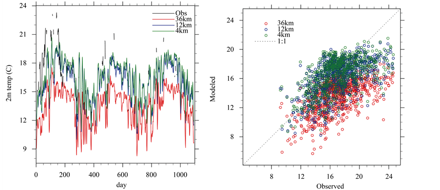
Metropolitan Mexico City occupies a large bowl-like depression ringed by mountains. Time series of temperatures for Mexico City for GSOD observations and from each of the three relevant AR5 model domains (Figure 2(a)) and scatterplots of model versus observations (Figure 2(b)) clearly show improvements with increased horizontal resolution. The 36 km model results are much colder than observations, while both the12 km and 4 km domains match up better. This behavior is reflected in the scatter plots, as the 12 km and 4 km model results lie largely atop one another, while the 36 km results are clearly offset. Comparing the station elevation to that of the nearest gridpoint in each of the three model domains (Table 2), it is clear that the 36 km results are colder because at that resolution the urban depression is not properly resolved?all that is picked up is the surrounding topographic heights.
Cali, Colombia is in the long, but narrow, Cauca Valley. Time series and scatterplots of temperature for GSOD and the three model domains for Cali (Figure 3) further exemplify the effect of topographic resolution.
 (a) (b)
Figure 2. Mexico City, Mexico temperature a) time series (5-day running average) and b) scatterplot.
Table 2. Verification statistics for selected stations.
 (a) (b)
Figure 3. Cali, Colombia temperature a) time series (5-day running average) and b) scatterplot.
Clearly, the 36 km domain is unable to resolve this deep valley, being far too cold. Both the 12 km and 4 km domains show quite good agreement with the observations, indicating that these finer spatial scales do suitably resolve the topographic depression within which Cali lies. Interestingly, the 12 km simulation is slightly too warm, as the gridpoint elevation is over 300 m below the actual station elevation. The 4 km simulation, while agreeing quite well with observations, also appears too low in elevation. Examining the reasons for this, it appears that the 30-second topographic dataset distributed with WRF has a region of lower elevation in the Cali region that does not appear in other topographic maps of the area, or in ground-level and aerial photos. In essence, the Cacua River Valley appears to be too deep in this dataset. Because the station elevation reported for Cali airport is higher than the model topography at 12 km and 4 km, the implication is that the WRF simulation is actually several degrees too cool for this location.
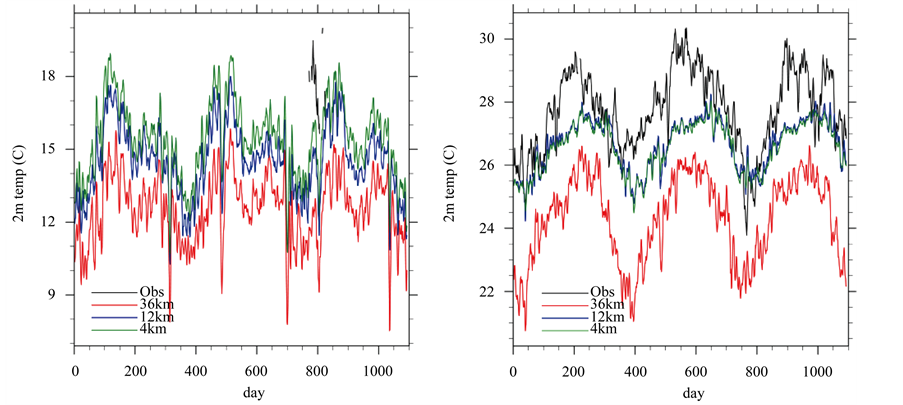
The results for Huehuetenango, Guatemala are more mixed (Figure 4(a)). This station is located partway up a mountainside, in a relatively flat bench-like area, with steeper slopes both above and below. Some effects of topography are clear, but they are more subtle than for Cali. Note also a key difficulty when attempting model observation comparisons―the observational record for Huehuetenango is extremely short for the three verification years―only 74 daily temperature observations are available. This points out the major difficulty in model validation in this region, as the ability to validate the model results is strongly dependent on the observational data available for the locale. Even though the station is at an elevation between that of the nearest gridpoints for the 12 km and 4 km domains, WRF has a clear cold bias at all three resolutions, although this bias is reduced with increasing resolution. Modeled temperature is also less variable than observed, resulting in significant underestimation of the high end of the observed temperature range. This may be the result of poor representation of the land use, as WRF specifies either dryland cropland and pasture (36 km) or evergreen needleleaf forest (12 km and 4 km), while satellite imagery from Google Earth indicates that the observation site is likely within the extensive built-up area of the city.
The results for Kingston, Jamaica (Figure 4(b)) show more significant differences. Kingston is an island city, located on the south coast of Jamaica, with low mountains inland to the north and east. The 36 km domain is much cooler than the station observations, while the 12 km and 4 km results are essentially identical, and somewhat cooler than observed. The nearest gridpoint in both the 12 km and 4 km domains are located over water, while the nearest gridpoint in the 36 km domain is over land, but on elevated terrain approximately 100 m above the observing station at the airport, located on a low-lying peninsula just above sea level.
These results demonstrate the importance of proper resolution of topography and surface type in simulating temperature. With global models, the concern has usually been resolving sufficient topographic heights. With higher resolution regional models and the ability to compare directly to station observations, a very different issue emerges. In general, humans do not build urban centers (with attendant meteorological stations) on top of
 (a) (b)
Figure 4. a) Huehuetenango, Guatemala and b) Kingston, Jamaica temperature time series (5-day running average).
mountains, but rather in valleys or broad depressions below. This means that a resolution that is too coarse will have an effective elevation that is too high, and simple lapse rate arguments support results that are too cold. Indeed, when comparing model to station observations, it may be necessary to choose the nearest gridpoint that is also closest to the station elevation, not necessarily the nearest gridpoint in an absolute geographic sense. Additionally, care must be taken to identify land use (especially land/water) representation in the model results, particularly for coastal locations and regions where significant patchiness in land cover exists.
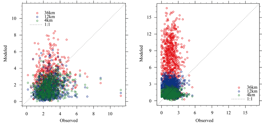
With the NNRP-driven simulation, WRF can be expected to simulate observed precipitation events. Indeed, for Mexico City (Figure 5), WRF captures many overall features. Basically, when the observations show rain, WRF results also show rain and at roughly the same magnitude for lesser events. WRF tends to have too many days with very small or even trace amounts of precipitation. This problem is ubiquitous in climate models, and usually is caused by insufficient evaporation of precipitation as it falls from the cloud in which it forms towards the surface. WRF also fails to capture the full magnitude of large events. When the observations show a lot of rain, WRF results also show it, just not quite so much (typically around 2/3rds of that observed). The higher resolution simulations appear to reproduce the distinct dry season that occurs in this region better than at 36 km.
Time series and scatter plots of precipitation for Cali (Figure 6) illustrate a potential problem with the GSOD data, as four days appear clearly to have observed precipitation that is much too high. We have compared the GSOD data to data from the Global Historic Climatology Network (GHCND), and it appears that GHCND better captures these events, suggesting that GSOD has problems with them. This requires further investigation that is beyond the scope of the study we describe here. Nonetheless, this makes comparison with WRF problematic, at least for Cali.
Kingston (Figure 7) shows quite good agreement overall at each resolution. The 36 km captures the one large observed event the best, while the 12 km and 4 km domains appear to do equally well at the numerous smaller events, both in timing and in magnitude.
Scatterplots for these three stations (Figure 5(b), Figure 6(b) and Figure 7(b)) indicate a possible “day of reporting” issue. Many stations report precipitation only once per day, often around 7 am local time (or anywhere from 11UTC to 15UTC across the expanse of these domains). As WRF output is set in UTC (and daily precipitation totals are accumulated at 00UTC for the preceding day) there can be a significant discrepancy in the reporting period between the model and observations. For example, if precipitation fell evenly over a 24-hour period at a station reporting at 12UTC (but locally 7 am), half the observed precipitation actually occurred on the previous day. Therefore, many rain events in WRF occur the day previous to when they show up in the observations, resulting in many plotted points on the scatterplot falling on one of the axes.
Statistical verification of precipitation is particularly problematic, as precipitation is decidedly not normally distributed and, thus, cannot be evaluated by the same measures as more normally distributed variables, such as
 (a) (b)
Figure 5. Mexico City, Mexico precipitation time series (a) and scatterplot (b).
 (a) (b)
Figure 6. Cali, Colombia precipitation time series (a) and scatterplot (b).
temperature and pressure. However, the ability of a model to correctly simulate the occurrence of precipitation (or precipitation exceeding a given amount) can be regarded in a dichotomous context, either the event did occur or it did not, and either the model did or did not simulate it. The results can be summarized in the classic 2x2 contingency table of hits (1), false alarms (2), misses (3), and correct rejections (4) from which various measures of model performance can be constructed [23] [24] . The Probability of Detection (POD) represents the proportion of occurrences that were forecasted correctly, i.e., POD = a/(a + c), while the False Alarm Rate (FAR) is the
 (a) (b)
Figure 7. Kingston, Jamaica precipitation time series (a) and scatterplot (b).
proportion of non-events that were forecasted to occur or FAR = b/(b + d). These two measures can be utilized to construct a simple diagram [25] that can give a visual representation of forecast skill (Figure 8). Using the converse of FAR, or Success Ratio (SR = 1 ? FAR), and POD as the two axes, a perfect forecast system would be plotted at the upper-left corner of the diagram. Moreover, two additional measures of forecast performance can be discerned in this diagram: frequency bias, the ratio of the number of forecasted events to the number of events observed [(a + b)/(a + c) = POD/SR] can be plotted as lines radiating from the origin; and Critical Success Index (CSI, sometimes called the threat score) [CSI = a/(a + b + c)] can be plotted, increasing outward on both axes. A bias greater than 1 (above the diagonal on the diagram) represents overforecasting, while a bias less than 1 represents underforecasting. CSI represents the proportion of correct forecasts, not counting correct rejections, and is a useful index when non-occurrence is much more frequent than occurrence. The improvement at all model resolutions when verifying 5-day rather than 1-day totals of precipitation is likely the result of the once-a-day reporting of precipitation noted above.
While winds throughout the free atmosphere in WRF are primarily determined by the large-scale NNRP (or GCM) forcing, the near-surface winds can be modified strongly by mesoscale weather features unresolved by the global model, local topography via conversion of horizontal motion to vertical and, to a lesser degree, by inhomogeneity in land cover. Figure 9 shows scatterplots (model versus observations) of wind speeds for Mexico City and Cali. For Mexico City, in all three domains the temporal pattern is well-simulated. The winds in the 36 km are invariably too strong, especially during high wind events. The winds in the 12 km domain, on the other hand, appear too weak, especially during low wind events. The winds in the 4 km domain overall appear to best represent the observations. The results for Cali are particularly striking. The 36 km domain has winds clearly much too strong; this problem also occurs most of the time in the 12 km domain, albeit not nearly as bad. The 4 km domain provides by far the best match overall. These results for Cali are not surprising, given the complexities of local topography described previously.
To provide quantitative measures for model-observation comparisons, standard verification statistics have been calculated, and summarized in Table 2. These include the mean, standard deviation, bias, mean absolute error (MAE), root mean square error (RSME), and correlation coefficient (CORR). Because of the importance of topography, the elevation and distance of the nearest WRF gridpoint relative to the station is given, along with the station elevation. Of particular interest is the bias, since reducing this is a primary objective of climate

Figure 8. Skill scores for all stations with more than 200 non-missing observations of precipitation computed for the 36 km (left), 12 km (middle) and 4 km (right) domains and for 1-day precipitation exceeding 2 mm (top) and 5-day precipitation exceeding 10 mm (bottom).
 (a) (b)
Figure 9. a) Mexico City, Mexico and b) Cali, Colombia wind scatterplots.
downscaling. For surface temperature, two items stand out. In every case except for Cali the bias is negative, that is, the model results are colder than observed (as described above, the positive bias results for Cali at 12 km and 4 km may well represent a mapping error). The second point is that in every case, the bias is reduced with increasing spatial resolution. This, of course, is why downscaling is performed. The standard deviation changes little with resolution (which may simply reflect that variability is expressed similarly on all scales) while the MAE and RSME decrease with increasing resolution, which indicates model improvement on a daily timescale as horizontal resolution increases. The correlation coefficients also change little as they are dominated by the seasonal cycle, which is faithfully captured by the data (i.e., reanalysis or GCM) used to force the downscaling.
The bias in precipitation also shows a reduction overall with increasing resolution. Indeed, at all stations except Cali the reduction between 36 km and 12 km is especially large. The results for Cali are more muddled, though as noted above, there are issues concerning station location. The bias changes in wind speed are mixed. For Cali and Huehuetenango, the bias decreases sharply between 36 km and 12 km resolution. On the other hand, the bias increases for Mexico City and Kingston with increasing resolution; the bias even changes sign for Kingston from an under-prediction at 36 km to large over-predictions at 12 km and 4 km. This suggests that local winds are problematic, especially in regions of complex topography.
3.2. How Well NNRP, CCSM4, and WRF Work?Seasonal Mean Climate
The comparison of the output from the NNRP-driven WRF simulation to station observations is the most direct way of evaluating model results. Nonetheless, the stations do not cover all regions, so evaluation of spatial climate patterns is also needed. In particular, stations tend to be located preferentially in populated lowland and valley regions. This means highland regions (and lowland sparsely populated regions such as Petén in Guatemala and Yucatan in Mexico) may be underrepresented. Analysis of mean climatic spatial patterns is also necessary for comparison to the CCSM4 control, as the mean patterns is all the latter can supply. We used monthly means to evaluate mean climate (as opposed to the daily weather evaluated using GSOD). Here, we show mean values averaged over the three-year (1991-1993) historic NNRP simulation, and averaged over the 5 year period “2006-2010” control from CCSM4 (the quote marks around 2006-2010 is a reminder that, unlike the NNRP simulation, the CCSM4 run does not simulate what actually occurred during this time period, but rather just a representative example of the full range of possibilities given greenhouse gas forcing representative of the period). The most basic results for seasonal temperature, precipitation, pressure, and winds at the surface are shown and discussed here.
The first step is to examine the results from the global scale NNRP. This is a bit of a “Catch-22” since these also serve as a primary observational proxy. All we can do is evaluate whether the basic climate patterns seem broadly reasonable at the large scale. Nonetheless, any obvious deficiencies in NNRP will likely carry over or be made worse when downscaled via WRF. The second step is to compare these results with those from NARR (over those regions where the WRF Mesoamerican domains and the NARR domain coincide). The final step is to evaluate results from WRF. Initial focus is on d01, since it roughly coincides in spatial resolution with NARR.
Figure 10 shows January and July temperature for the three-year 1991-1993 average, from NNRP, NARR, and WRF d01, all plotted on the WRF d01 domain. The temperature patterns in NNRP over land appear realistic, showing the effects of both seasonality and topography. Northern Mexico is quite cool during the winter season at those relatively higher latitudes, while at lower latitudes the effects of topography are obvious. Note also the warm pools over the eastern Pacific and western Atlantic. In July, the effects of topography are even more apparent, since this is a warm season throughout most of the region (minimum seasonality). NARR and the NNRP- driven WRF simulations show general large-scale features similar to the NNRP though the effects of the higher resolution (32 km for NARR; 36 km for WRF) are also obvious.
Figure 11 and Figure 12 are the same as Figure 10 but for the 12 km d02 domain and the 4 km d03 domain, respectively. The same basic temperature patterns are seen at 36 km and 12 km as in NNRP, but the effects of increasing spatial resolution become apparent at 12 km, where specific mountain ranges such as the Sierra Madre complex in Mexico are apparent. The results are most striking at 4 km resolution, where effects on temperature due to individual mountain peaks and valleys become obvious.
Figure 13 is similar to Figure 10 except it shows January and July precipitation for 1991-1993. The seasonal shifts are especially prominent, and as with temperature, realistic. The Intertropical Convergence Zone (ITCZ) is apparent in both seasons, though larger and more continuous in July. Poleward of the ITCZ (e.g, Mexico), precipitation minimizes in winter and maximizes in summer. Overall, the patterns appear reasonable.
Figure 14 and Figure 15 are the same as Figure 11 and Figure 12, but for precipitation. The effects of increased resolution are quite apparent, especially at 4 km, where the topographic highs and lows are delineated, though not as clearly as with surface temperature. Physically, these changes make sense relative to what would

Figure 10. Monthly climatological mean temperature for January (left) and July (right) 1991-1993 plotted over domain 01 for NNRP (top row), NARR (second row), and WRF d01 (bottom row).
be expected with enhanced resolution of topographic windward and leeward effects. Validating this enhanced performance with increasing resolution is problematic as the lack of observations beyond the GSOD point station measurements employed above means we cannot be certain that the enhanced spatial detail represents an actual improvement. It is clear, however, that topographic effects are better resolved.
While surface temperature and precipitation may be of most importance for impacts studies, both are strongly dependent on the underlying atmospheric pressure and wind patterns. The large-scale pressure patterns (not shown) are similar in all cases, and largely reflect seasonal shifts in the ITCZ. More detail is seen at higher resolutions, but this is indicative of the elevation-dependent reduction from surface pressure to equivalent sea level pressure. The near-surface winds (not shown) are consistent with these pressure patterns, though at the 12 km and 4 km resolution domains in WRF the trade winds are restricted to the immediate Atlantic coast with light and variable winds over the interior and Pacific coasts. This latter feature is especially important for scenarios of future climate change.
The final step is to examine the global model used to drive WRF (NCAR CCSM4) for the climate change simulations, to see how well it represents the present-day climate of the region, especially in comparison to the “proxy” NNRP observations presented above (see also [22] for a global perspective). As for NNRP, this comparison is for both stand-alone CCSM4 results and results when WRF is driven by forcing from CCSM4. Figure 16 is similar to Figure 11, but for 2006-2010 and with the CCSM4 results also included. The spatial patterns and the magnitudes over land compare quite well to the 5-year climatology from the NNRP reanalyses. In the WRF simulations, this increased detail, not surprisingly, follows mostly the topography, with a lesser component due to coastal versus non-coastal effects.
Figure 17 shows precipitation for January and July over domain d02. Here the agreement is not as good. At the broadest scale, there is correspondence in spatial patterns, but the GCM has less detail, and maximum amounts are also less. In particular, the location of the ITCZ is well-handled, but the amounts overall are too low, especially over Panama in January and the Amazon basin in July. The GCM also appears to lack sufficient seasonality over both ocean and land. In the WRF simulations, these deficiencies largely carry though, as they

Figure 11. Monthly climatological mean temperature for January (left) and July (right) 1991-1993 plotted over domain 02 for NNRP (top row), NARR (second row), WRF d01 (third row), and WRF d02 (bottom row).
represent deficiencies in the large-scale forcing that WRF is unable to overcome. What WRF clearly can do is account for the effects of topography on precipitation, though, as above, it is hard to verify that this does indeed represent a real improvement.
As an overall summary, the GCM appears to replicate the observed climatological features fairly well. There is some question about precipitation, but it is also not clear how well this is captured by the reanalyses. Similar to the NNRP simulations, the enhancements in the WRF simulations are clearly dependent on the better resolution of topography.
3.3. Future Climate Changes
Focus is on basic results for differences in surface temperature and precipitation, as these are the variables typically most important for vulnerability and impacts studies (e.g., [4] - [6] ). Here, we present the CCSM4 and WRF climatological differences between the present-day and mid-century periods, over WRF domain d02 (Figure 18, Figure 19). We address two specific questions: 1) How do the downscaled WRF results differ overall from the GCM in spatial pattern and in magnitude; and 2) What are the significant differences in resolution between 12 km and 4 km, how are these region specific (e.g. those with complex topography, versus those with less relief, such as coastal plains), and do they represent improvements? The results below are grouped by variable: surface temperature, then precipitation, sea level pressure, and finally surface winds.
Figure 18 shows the five-year mean surface temperature change (2056-2060) minus the control (2006-2010), for January and July for CCSM4 and WRF, the latter for the 12 km d02. Roughly similar patterns of warming are seen in both seasons, as much as 3˚C - 4˚C over the larger landmasses of Mexico and northern South America, reducing to 0.5˚C - 1.5˚C over the isthmus of Central America, and the Caribbean islands of Hispaniola and

Figure 12. Monthly climatological mean temperature for January (left) and July (right) 1991-1993 plotted over domain 03 for NNRP (top row), NARR (second row), WRF d01 (third row), WRF d02 (fourth row), and WRF d03 (bottom row).
Puerto Rico.
Overall, large-scale patterns of the downscaled results from WRF do not differ significantly from those obtained from the global model alone (e.g., [10] ). What is clear, however, is the small-scale, additional detail obtained at higher resolutions. For example, maximum differences in temperature for CCSM4 tend to be concentrated in a few bulls-eyes, such as in northwestern Mexico and in the northern Amazon basin. These are also found in the higher resolution WRF d01 and d02, but with additional detail, especially apparent in the 12 km d02. The 4 km domain (d03) over central and southern Mexico and northern Central America demonstrates this even more. The 4 km domain over Hispaniola and Puerto Rico (d04) on the other hand, provides little additional information relative to the 12 and 36 km domains, or for that matter, the large-scale GCM forcing. It appears that even though these islands contain steep topographic features, overall the area is quite small, and the climate changes are dominated by what occurs over adjacent ocean regions. Recall that WRF does not directly simulate sea surface temperature changes; instead they are interpolated from the GCM forcing to the resolution of the WRF domain. Overall, the temperature differences are largely indifferent to season; that is, the results and their implications differ little from January to July.

Figure 13. Monthly climatological total precipitation for January (left) and July (right) 1991-1993 plotted over domain 01 for NNRP (top row), NARR (second row), and WRF d01 (bottom row).

Figure 14. Monthly climatological total precipitation for January (left) and July (right) 1991-1993 plotted over domain 02 for NNRP (top row), NARR (second row), WRF d01 (third row), and WRF d02 (bottom row).
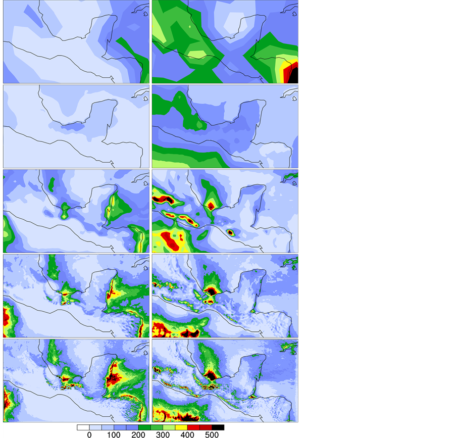
Figure 15. Monthly climatological total precipitation for January (left) and July (right) 1991-1993 plotted over domain 03 for NNRP (top row), NARR (second row), WRF d01 (third row), WRF d02 (fourth row), and WRF d03 (bottom row).
Figure 19 is the same as Figure 18, except now for precipitation. Because of the wide range of absolute precipitation values across the region, differences are shown as per cent change relative to the mean for each point. Focusing first on CCSM4 for January, generally fairly small changes are seen throughout the region, with slight increases for northern Central America and the Pacific coast of Colombia, with little change or small decreases elsewhere. This is not unexpected, as most of the region is in a dry season during January. In July, the same general pattern is seen for Central America and the Pacific coast of Colombia, though the changes are larger during what is now a wet season month. Much of Mexico and the remainder of Colombia now see an increase. Though not explicitly reported on by Meehl et al. [22] , it is also possible that the future simulation contains an ENSO event that does not occur in the present-day case [26] .
Especially important here are the differences in SLP for the global model, as WRF should maintain fidelity to this large-scale phenomena. The changes are subtle, but nonetheless meaningful. In January, there is a meridional shift in sea level pressure, with slightly lower pressure to the east and higher to the west. In July, pressures increase slightly almost everywhere. In combination, these indicate an expansion of the subtropical high zones,

Figure 16. Monthly climatological mean temperature for January (left) and July (right) 2006-2010 plotted over domain 02 for CCSM4 (top row), NNRP (second row), NARR (third row), and WRF d02 (bottom row).
with relaxation of both the Trade Wind and Walker circulations and consequent impacts [22] . For the specific smaller domains, though, as expected, the same large-scale features prevail. The key point is that SLP is little changed in WRF, but local topographic features then take these basic pressure patterns and their differences and significantly modify the surface winds, as described below.
The results for temperature and especially precipitation are suggestive of potentially significant changes in the low-level circulation. Furthermore, some subtle but important patterns were seen in the global model for SLP differences. The WRF results display these same patterns; what differences are seen again highlight the topography. In this case, however, these differences probably are not physical, reflecting instead the strongly elevation-dependent reduction of surface pressure to sea level. What is important is that WRF appears to faithfully capture the large-scale differences in the pressure field. At the local and regional scale, it is the surface winds that are most important for impact and vulnerability studies.
The GCM and low resolution (36 km) WRF in general have the trade winds blowing too strongly across southern Mexico and Central America. This is due to poor resolution of topography, as the problem is lessened, but still persists in d02. The trade winds, which are little changed in January (during the time of winter minimum in the Northern Hemisphere), show a sharp decrease across the entire region in July. The changes in the higher resolution domains also indicate that the trade winds in January may decrease slightly over interior and Pacific coastal regions. These changes are consistent with those noted above in sea level pressure. The importance is that these trade wind related features occur across much of the region. In particular, at 4 km resolution, the wind
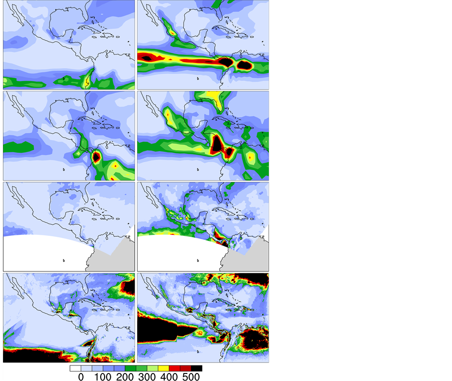
Figure 17. Monthly climatological total precipitation for January (left) and July (right) 2006-2010 plotted over domain 02 for CCSM4 (top row), NNRP (second row), NARR (third row), and WRF d02 (bottom row)
patterns are more realistic, reflecting the blocking of low-level trade winds by topographic features. The wind differences clearly indicate that at the 12 km and 4 km higher resolutions, the changes in winds are quite small and variable over the interior and along the Pacific coastal regions. The largest reductions are restricted to the Atlantic coast, especially from Yucatán Peninsula through central Panama.
Summarizing key results, the MAC everywhere warms; the warming is larger with higher topographic elevations and distance from the coast. The results for precipitation are less straightforward. A general decrease occurs along the Atlantic coast of Central America, consistent with a weakening of the trade winds. Elsewhere little difference, or even a slight increase occurs. This is at odds with the GCM and 36 km WRF results in which the trade winds blow from the Atlantic to the Pacific, instead of being mostly blocked by mountains near the Atlantic coast. A resolution of 12 km appears sufficient to resolve this latter effect, though it is also clear that in the mountainous regions, the 4 km provides more realistic details. These results demonstrate the importance of horizontal spatial resolution sufficient to resolve the effect upon climate of topographic features, as well as the nature over the underlying landscape.
4. Discussion
The purpose of this study is to develop a strategy and mechanism for providing high-resolution results for the remainder of this century for Mesoamerica under an assumed scenario of future climate change. Motivation was

Figure 18. Monthly climatological mean temperature difference for January (left) and July (right) plotted over domain 02 for CCSM4 (top row) and WRF d02 (bottom row).
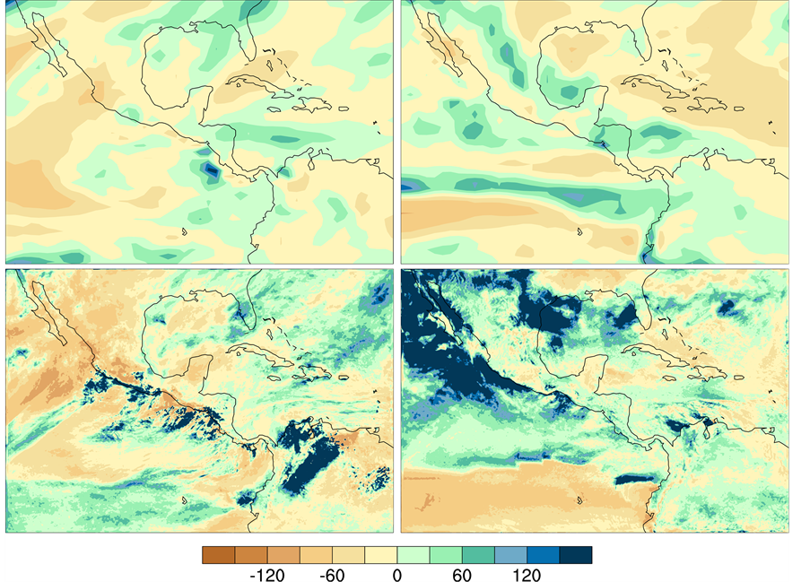
Figure 19. Monthly climatological percentage precipitation difference for January (left) and July (right) plotted over domain 02 for CCSM4 (top row) and WRF d02 (bottom row).
provided by the need for reliable information at the spatial scale required for national climate assessment plans and other local vulnerability and adaptation studies [4] - [6] .
4.1. Model Verification
Key results include: 1) Accuracy of the temperature simulation is strongly dependent on altitude. If topographic features are not properly resolved, upland regions are simulated to be too warm, while lower elevation regions (where most human occupation occurs and, hence, most reporting stations are located) are simulated to be too cold. In regions of complex topography (such as occupy much of the region), a resolution of 4 km is necessary to properly capture these effects. In larger, more homogeneous regions, such as the basin in which Mexico City is located, 12 km may be sufficient. This also applies to Kingston, Jamaica, which, though located on a coastal plain, is backed by low inland mountains. For broad coastal plains lacking in nearby topography, such as Tocumen, Panama, for example, and which are strongly conditioned by the adjacent ocean, 36 km may suffice. The same applies to small Caribbean islands. Such locations are, however, rare throughout Mesoamerica as a whole.
2) Precipitation and wind are much more complex fields and hence more difficult to simulate. Furthermore, lack of sufficient observational data, especially at suitable spatial scales, is a major impediment for verification. Nonetheless, a few general conclusions can be drawn. The CCSM4 broadly captures overall precipitation features, but spatial details are lacking, and magnitudes are generally underestimated, especially in regions with considerable precipitation. Evaluation of the winds also points to a systemic problem in which, due to insufficient resolution of topography along the immediate Atlantic coast, the northeast trade winds blow unimpeded from the Atlantic across the isthmus of Central America towards the Pacific. This places the entire region under a regime of trade wind precipitation, while in reality the low (1 - 1.5 km elevation) mountains along the Atlantic coast are sufficiently high to largely block the trade wind flow and attendant precipitation. This will be of major significance when evaluating model simulations of future climate change for the region.
3) The comparison of actual weather events to mean climate for the region helps support the robustness of the model results. WRF was able to simulate quite well the actual station surface temperatures observed from 1991- 1993, especially when the station elevation was properly resolved. Precipitation was also generally well simulated. That is, when it rained at reporting stations, it also rained in the NNRP-driven WRF simulation. This was especially apparent for large precipitation events, though WRF did tend to underestimate the magnitude (generally giving amounts about 2/3rds of those observed). In part this may be due to WRF representing an average that even at 4 km resolution (i.e., 16 km2) cannot capture the full amount of a point measurement made at a station. A more robust observational database would be required to resolve this issue.
4) The climate simulated by CCSM4 is not as robust as that provided by the quasi-observational NNRP. This is to be expected, as the GCM solves for the climate based solely on basic physical principles and imposed external forcings (which may or may not be well-known). NNRP on the other hand, while at the core based on a model similar to the GCM, also assimilates all available observational data, which presumably means it gives a more realistic simulation. In the event, we have no realistic alternative but to consider NNRP as “ground-truth”. WRF appears able to compensate for some of the known GCM deficiencies (e.g., the poor handling of the trade winds) but may not be able to cope as well with others. This must be borne in mind when evaluating use of WRF climate change simulations.
4.2. Future Climate Changes
The global model CCSM4 results show a warming over all of Mesoamerica between the present and the 2050’s, ranging from less than 1˚C to in excess of 3˚C. The largest warming occurs over interior and highland regions, while coastal regions show the least change. These same general patterns hold with the high resolution downscaling, though additional detail and important changes are seen. In particular, the effects of topography are much better resolved. As a particularly striking example, the patterns of surface temperature difference largely follow the topography. Indeed, the more realistic representation of topography with increasing resolution is clearly indicated by the surface temperature results?one could almost use them as a proxy for topography. Coastal regions show lesser change, presumably because of the strong ocean influence. Following basic thermodynamic principles and, as all previous climate modeling studies have indicated, the upper ocean responds less quickly than the overlying atmosphere, due to its thermal inertia. This means simulated coastal temperature changes are muted relative to those over interior land regions. Furthermore, SST in the WRF simulations are not calculated, but rather obtained via interpolation from the driving large-scale GCM simulations.
The global model results for precipitation are more at odds with those from WRF, reflecting in turn a more complex situation [27] - [29] . Topography has a strong, direct influence on precipitation, as it does with temperature. Over windward slopes air is forced to rise, enhancing condensation and precipitation, while over leeward slopes, air descends, inhibiting precipitation. This direct signal can clearly be seen in the high-resolution results shown above. But, as described in more detail below, changes in the overall wind regime are also important. In actuality trade wind precipitation is restricted to the immediate Atlantic coast, while in GCM simulations it is able to spread across the entire Central American isthmus from the Gulf of Tehuantepec to the Darien Gap. This implies a trade wind precipitation regime for the entire region, with a future decrease consistent with the relaxation of the latitudinal temperature gradient and hence driving force for the trade winds. This is indeed seen in the GCM simulations. These differences can be clearly seen in comparing the CCSM4 versus WRF results. The results for precipitation from WRF are very different than those from the GCM, and are consistent with better resolution of topographic effects, especially along the Atlantic coast.
Two major themes emerge. The first is the degree to which better resolution of the land surface, especially its topography, enables WRF to take the large-scale, broadly reasonable GCM results and “downscale” them to enable more realistic local effects on temperature, precipitation, and winds. This is what we normally associate with a downscaling process, be it dynamical or statistical. Indeed, the results described above clearly indicate both the effects of topography and proximity to the oceans (coastal regions).
A second theme emerges―the GCM is unable to properly simulate the trade wind regime over Mesoamerica, due to insufficient resolution of the low mountains along the Atlantic coast that in reality are sufficiently high to largely block the passage of the trade winds inland. These subtropical and tropical latitudes are in general strongly influenced by the trade winds, that is, winds blowing anticyclonically from higher latitudes towards the equator (i.e., from subtropical high pressure towards the low pressure of the ITCZ). Over oceans these winds blow largely unchecked. Over land, frictional effects retard the winds; these low level winds (typically confined to 1 - 2 km above the surface) are further blocked by the low mountain range (1 - 1.5 km) that lines much of the Atlantic coast of Mesoamerica.
This effect is, however, captured in the WRF simulations, at both 12 km and 4 km resolution. In this case, the downscaling is able to take a large-scale forcing associated with changes in the trade winds and simulate instead a very different precipitation regime for inland and Pacific coast regions of Mesoamerica. This regime in WRF involves convection developing over the eastern Pacific and then drifting eastward over adjacent land regions. The key is that all climate models suggest a relaxing of the trade winds with a warmer future world, with an accompanying reduction in precipitation. In the global models, this translates to a reduction in precipitation over all land regions. In the WRF results, on the other hand, the trade winds and associated precipitation are restricted to the immediate Atlantic coast. Over the remainder of the region, however, the drifting ashore of convection from the eastern Pacific appears largely unchanged into the future.
4.3. Model Uncertainties―How Much Can We Trust These Climate Change Results?
Two distinct types of uncertainty can be identified. The first of these concerns the long term signal versus the short term noise due to interannual to decadal scale variability. When using coupled models for dynamical downscaling (or other purposes) this type of uncertainty cascades, in an as yet poorly understood fashion. This uncertainty can perhaps be best understood in terms of a standard error, that is, a statistical representation of the unbiased variability.
The second uncertainty concerns model biases, as well as the lack of two-way interaction. A primary goal of downscaling is to reduce biases that occur at the large spatial scale (100 km or greater) relative to the local or regional scale (10 - 15 km or less). This goal is sometimes met with the 12 km domain, and almost always met with a 4 km domain (Table 2). A key issue concerns bias versus variance―is the reduction in bias justified given the increase in variance? We do not provide definitive answers here but raise the issue, and have a study underway to explore this further.
Uncertainty in future climate projections reflects these two uncertainties, as well as uncertainties regarding future changes (e.g., emission scenarios). We chose RCP8.5 precisely because it represents the largest reasonable change expected over the remainder of the 21st century. Once these climate change boundaries are established, any true scenario that involves lesser emissions will presumably induce a smaller response in climate. An additional issue concerns distinguishing the “signal” due to increased greenhouse gases as it unfolds over the remainder of this century from the “noise” due to interannual and decadal scale variability inherent in the climate system (e.g., as measured by the standard error above). The most robust modeling strategy targeting this issue would involve ensembles of WRF runs driven by CCSM4 for the entire period 2006-2100. Unfortunately, due to computational, data storage, and human resource issues, such an approach is not feasible, at least at this time. Given a choice between multiple simulations at moderate (25 - 50 km) spatial resolution or making a very few simulations at high resolution (4 - 12 km), as described in Section 2, we chose the latter approach.
4.4. Implications for Vulnerability and Adaptation Studies
The motivation behind this work is to understand better the implications of these potential climate changes for human and natural resources and systems in Mesoamerica. While this is a topic of considerable need by itself that will be addressed specifically in future studies, some broad conclusions can be drawn from this basic climate change research. Our simulations results show temperatures increase everywhere, with the effects greatest in highland regions and less in coastal regions. While heat waves are likely to increase everywhere in this tropical and subtropical region, the fact that they are less prevalent in the relatively cooler highlands will mitigate the effects due to future warming. The warmer temperatures will lead to greater evapotranspiration stress, which could have detrimental effects on human activities, especially agriculture. Water resources for human consumption and other economic activities, as well as biodiversity, especially native flora and fauna, could also become stressed.
This stress also means effective drying, even without precipitation reductions. Along the Atlantic coast of Central America, the results show that precipitation in general will decrease; however this is a region that is typically wet, with generally ample water resources at present. Thus the combination of increased evaporative stress and reduced precipitation in the future may have less impact over this region. Over much of the remaining region, precipitation is relatively unchanged. The warming may lead to some overall effective drying, but, as long as proper long-term planning considers appropriate adaptation strategies, water resources, such as availability for hydroelectric power generation, may not suffer severe effects. Precipitation intensity likely increases when it does rain, as the warmer atmosphere can hold more moisture, which may in turn, however, increase the likelihood of river flooding events. These river floods, as well as other extreme events such as heat waves and coastal flooding, are the topic of a separate study currently underway. Furthermore, Oglesby et al. [30] showed that local deforestation may have more severe consequences than AGW on the regional hydrologic cycle and, hence, water resources.
5. Conclusions
MAC has been identified as a low-latitude region at particular risk for the effects of climate change. Global climate models can provide a large-scale assessment of the basic climate drivers, but cannot account for the local effects of topography and land use, which in turn strongly impact temperature and precipitation. To help overcome this problem, the WRF regional model was used to downscale CMIP5 results from the NCAR CCSM4 global model at 4 - 12 km resolution for Mesoamerica and the Caribbean. To evaluate WRF, a three-year “historic” run forced by NCEP/NCAR reanalyses was made for 1991-1993 and was compared to station observations, in order to identify WRF biases. Because the large-scale forcing is constructed from the weather that actually occurred, this simulation can be compared directly with station observations. Two five-year runs were made with WRF forced by CCSM4, one for the “present-day” (2006-2010) and one for projected climate changes 50 years into the future (2056-2060). The former simulation can also be used for model verification, and is used here for that purpose.
Because of the very strong impact of topography on surface temperature, the results clearly demonstrate the need for high resolution in order for it to be properly simulated. Land use changes (especially urbanization) may also play an important, though secondary, role. Precipitation is more difficult to evaluate, being composed of discrete events highly variable in time and space (as opposed to the much smoother, continuous temperature). When it rains at a GSOD station, in most instances WRF also has a rainy event. WRF also does a reasonable job of simulating large rain events when they actually occur, though it does tend to underestimate the magnitude. Additionally, WRF produces too many low-rainfall days (a problem shared with most climate models). Simulation of the surface winds tends to be too strong at 36 km resolution and much improved at 12 km and, especially, 4 km. Importantly, a suite of standard verification statistics are computed and show that the biases are sharply reduced at higher resolutions, while standard errors are little changed.
The simulation of the large-scale mean seasonal climate is reasonable in NNRP and in CCSM4, especially for surface temperature. Large-scale precipitation spatial patterns also appear reasonably well simulated although the magnitudes in the GCM appear to be underestimated. The effects of the higher-resolution WRF domains include much more realistic local output, conforming especially to topography, while also maintaining large-scale fidelity. Lack of suitable observations precludes quantitative evaluation of how much of an improvement this represents. The surface pressures and winds appear to be reasonably well simulated. Overall, the CCSM4/WRF combination appears to adequately simulate the preset-day climate of Mesoamerica, lending credence to its ability to simulate future climate change in coming decades. It is a goal of this study that these results should be used by each individual country of Mesoamerica to help them better identify their future vulnerabilities to a changing climate, and to provide guidance in the development of national and local adaptation strategies.
Those differences between simulations have shown that all regions will warm; in general the warming is larger with higher topographic elevations and distance from the coast, such as the western Amazon basin. Surrounding ocean waters moderate the warming over the Caribbean islands. A resolution of 4 km is required to properly resolve temperatures in regions of complex topography, while 12 km may be sufficient for lowland, coastal, and island regions. The results for precipitation are less straightforward. In general a decrease occurs along the Atlantic coast, where pressure and wind changes suggest a weakening of trade wind-induced precipitation. Elsewhere, changes are mixed, with much of the region seeing little difference, or even a slight increase. This is at odds with the GCM and 36 km WRF results, but at these lower resolutions, the trade winds blow from the Atlantic to the Pacific, instead of being blocked by mountains near the Atlantic coast. A resolution of 12 km appears sufficient to resolve this latter effect.
The next steps include: 1) Global warming due to increased greenhouse gas emissions is not the only potential agent of climate change. Studies suggest that temperature changes due to land use alterations may be as large, at least locally [30] . Atmospheric aerosols, even if generated from afar, may also play a role. A key goal remains quantifying the relative impacts of competing processes, particularly the effects of deforestation; 2) Further evaluating the degree of topographic complexity required―is 4 km resolution sufficient? What benefits, if any, are provided by increasingly higher resolution? What is the relationship between explicit resolution of convection and microphysics parameterization schemes at higher resolutions? 3) Can our modeling strategy be fine- tuned, or adapted to the changing software and hardware configurations prevalent in climate modeling? 4) How best to use these results to provide robust input into regional and national climate assessments? Such usage ultimately is the primary purpose of this research.
Acknowledgements
This work was funded by generous support from the Sustainable Energy and Climate Change Initiative of the Inter-American Development Bank. Computational resources were provided by the Holland Computing Center of the University of Nebraska, while the Center for Water in the Humid Tropics of Central America and the Caribbean (CATHALAC) provided valuable logistical support. We also acknowledge our partner organizations in the countries of Mesoamerica and the Caribbean, who provided support for the participation of our coauthors.
Cite this paper
Robert Oglesby,Clinton Rowe,Alfred Grunwaldt,Ines Ferreira,Franklyn Ruiz,Jayaka Campbell,Luis Alvarado,Francisco Argenal,Berta Olmedo,Alejandro del Castillo,Pilar Lopez,Edwards Matos,Yosef Nava,Carlos Perez,Joel Perez, (2016) A High-Resolution Modeling Strategy to Assess Impacts of Climate Change for Mesoamerica and the Caribbean. American Journal of Climate Change,05,202-228. doi: 10.4236/ajcc.2016.52019
References
- 1. UNFCCC (2007) Vulnerability and Adaptation to Climate Change in Small Island Developing States. United Nations Framework Convention for Climate Change, Bonn.
- 2. Kasa, S., Gullberg, A.T. and Heggelund, G. (2008) The Group of 77 in the International Climate Negotiations: Recent Developments and Future Directions. International Environmental Agreements: Politics, Law and Economics, 8, 113- 127.
http://dx.doi.org/10.1007/s10784-007-9060-4 - 3. IPCC (2007) Climate Change 2007: The Physical Science Basis. Contributions of Working Group I to the Fourth Assessment Report of the Intergovernmental Panel on Climate Change [Solomon, S., Qin, D., Manning, M., Chen, Z., Marquis, M., Averyt, K.B., Tognor, M. and Miller, H.L., Eds.]. Cambridge University Press, United Kingdom and New York, NY, USA, 996 p.
- 4. IPCC (2007) Climate Change 2007: Impacts, Adaptation, and Vulnerability. Contribution of Working Group II to the Fourth Assessment Report of the Intergovernmental Panel on Climate Change [Parry, M.L., Canziani, O.F., Palutikof, J.P., van der Linden, P.J. and Hanson, C.E., Eds.]. Cambridge University Press, United Kingdom and New York, NY, USA, 976 p.
- 5. IPCC (2013) Climate Change 2013: The Physical Science Basis. Contribution of Working Group I to the Fifth Assessment Report of the Intergovernmental Panel on Climate Change [Stocker, T.F., Qin, D., Plattner, G.-K., Tignor, M., Allen, S.K., Boschung, J., Nauels, A., Xia, Y., Bex, V. and Midgley, P.M., Eds.]. Cambridge University Press, Cambridge, United Kingdom and New York, NY, USA, 1535 p.
- 6. IPCC (2014) Climate Change 2014: Impacts, Adaptation, and Vulnerability. Part B: Regional Aspects. Contribution of Working Group II to the Fifth Assessment Report of the Intergovernmental Panel on Climate Change [Barros, V.R., Field, C.B., Dokken, D.J., Mastrandrea, M.D., Mach, K.J., Bilir, T.E., Chatterjee, M., Ebi, K.L., Estrada, Y.O., Genova, R.C., Girma, B., Kissel, E.S., Levy, A.N., MacCracken, S., Mastrandrea, P.R. and White, L.L., Eds.]. Cambridge University Press, Cambridge, United Kingdom and New York, NY, USA, 688.
- 7. Taylor, M.A., Whyte, F.S., Stephenson, T.S. and Campbell, J.D. (2011) Why Dry? Investigating the Future Evolution of the Caribbean Low Level Jet to Explain Projected Caribbean Drying. International Journal of Climatology, 33, 784- 792.
http://dx.doi.org/10.1002/joc.3461 - 8. Campbell, J.D., Taylor, M.A., Stephenson, T.S., Watson, R.A. and Whyte, F.S. (2011) Future Climate of the Caribbean from a Regional Climate Model. International Journal of Climatology, 31, 1866-1878.
http://dx.doi.org/10.1002/joc.2200 - 9. Martínez-Castro, D., Porfirio da Rocha, R., Bezanilla-Morlot, A., Alvarez-Escudero, L., Reyes-Fernández, J.P., Silva- Vidal, Y. and Arritt, R.W. (2006) Sensitivity Studies of the RegCM3 Simulation of Summer Precipitation, Temperature and Local Wind Field in the Caribbean Region. Theoretical and Applied Climatology, 86, 5-22.
http://dx.doi.org/10.1007/s00704-005-0201-9 - 10. Diro, G.T., Rauscher, S.A., Giorgi, F. and Tompkins, A.M. (2012) Sensitivity of Seasonal Climate and Diurnal Precipitation over Central America to Land and Sea Surface Schemes in RegCM4. Climate Research, 52, 31-48.
http://dx.doi.org/10.3354/cr01049 - 11. Karmalkar, A.V., Bradley, R.S. and Diaz, H.F. (2008) Climate Change Scenario for Costa Rican Montane Forests. Geophysical Research Letters, 35, L11702.
http://dx.doi.org/10.1029/2008gl033940 - 12. Hernandez, J.L., Srikishen, J., Erickson, D.J., Oglesby, R.J. and Irwin, D. (2006) A Regional Climate Study of Central America Using the MM5 Modeling System: Results and Comparison to Observations. International Journal of Climatology, 26, 2161-2179.
http://dx.doi.org/10.1002/joc.1361 - 13. Centella, A., Bezanilla, A. and Leslie, K. (2008) A Study of the Uncertainty in Future Caribbean Climate Using the PRECIS Regional Climate Model. Technical Report, Community Caribbean Climate Change Center, Belmopan, 16 p.
- 14. Ruiz, F. (2010) Cambio climático en temperatura, precipitacion y humedad relativa para Colombia usando modelos meteorológicos de alta resolucion (Panorama 2011-2100). Nota Técnica del IDEAM, IDEAM-METEO/005-2010.
http://modelos.ideam.gov.co/media/dynamic/escenarios/nota-tecnica-sobre-generacion-de-ecc.pdf - 15. Van Vuuren, D.P., Edmonds, J., Kainuma, M., Riahi, K., Thomson, A., Hibbard, K., Hurtt, G.C., Kram, T., Krey, V., Lamarque, J.-F., Masui, T., Meinshausen, M., Nakicenovic, N., Smith, S.J. and Rose, S.K. (2011) The Representative Concentration Pathways: An Overview. Climatic Change, 109, 5-31.
http://dx.doi.org/10.1007/s10584-011-0148-z - 16. Riahi, K., Rao, S., Krey, V., Cho, C., Chirkov, V., Fischer, G., Kindermann, G., Nakicenovic, N. and Rafaj, P. (2011) RCP8.5—A Scenario of Comparatively High Greenhouse Gas Emissions. Climatic Change, 109, 33-57.
- 17. Racherla, P.N., Shindell, D.T. and Faluvegi, G.S. (2012) The Added Value to Global Model Projections of Climate Change by Dynamical Downscaling: A Case Study over the Continental U.S. Using the GISS-ModelE2 and WRF Models. Journal of Geophysical Research, 117, D20118.
http://dx.doi.org/10.1029/2012JD018091 - 18. Skamarock, W.C., Klemp, J.B., Dudhia, J., Gill, D.O., Barker, D.M., Duda, M.G., Huang, X-Y., Wang, W. and Powers, J.G. (2008) A Description of the Advanced Research WRF Version 3. NCAR Technical Note NCAR/TN-475+STR, 113 p.
- 19. Lo, J.C.F., Yang, Z.-L. and Pielke Sr., R.A. (2008) Assessment of Three Dynamical Climate Downscaling Methods Using the Weather Research and Forecasting (WRF) Model. Journal of Geophysical Research, 113, D09112.
http://dx.doi.org/10.1029/2007jd009216 - 20. Kalney, E., Kanamitsu, M., Kistler, R., Collins, W., Deaven, D., Gandin, L., Iredell, M., Saha, S., White, G., Woollen, J., Zhu, Y., Leetmaa, A., Reynolds, R., Chelliah, M., Ebisuzaki, W., Higgins, W., Janowiak, J., Mo, K.C., Ropelewski, C., Wang, J., Jenne, R. and Joseph, D. (1996) The NCEP/NCAR 40-Year Reanalysis Project. Bulletin of the American Meteorological Society, 77, 437-471.
http://dx.doi.org/10.1175/1520-0477(1996)077<0437:TNYRP>2.0.CO;2 - 21. Gent, P.R., Danabasoglu, G., Donner, L.J., Holland, M.M., Hunke, E.C., Jayne, S.R., Lawrence, D.M., Neale, R.B., Rasch, P.J., Vertenstein, M., Worley, P.H., Yang, Z.-L. and Zhang, M. (2011) The Community Climate System Model Version 4. Journal of Climate, 24, 4973-4991.
http://dx.doi.org/10.1175/2011JCLI4083.1 - 22. Meehl, G.A., Washington, W.M., Arblaster, J.M., Hu, A., Teng, H., Tebaldi, C., Sanderson, B.N., Lamarque, J.-F., Conley, A., Strand, W.G. and White III, J.B. (2012) Climate System Response to External Forcings and Climate Change Projections in CCSM4. Journal of Climate, 25, 3661-3683.
http://dx.doi.org/10.1175/JCLI-D-11-00240.1 - 23. Wilks, D.S. (2011) Statistical Methods in the Atmospheric Sciences. 3rd Edition, Academic Press, Oxford.
- 24. Jolliffe, I.T. and Stephenson, D.B. (2012) Forecast Verificaton: A Practitioner’s Guide in Atmospheric Science. 2nd Edition, Wiley-Blackwell, Oxford.
- 25. Roebber, P.J. (2009) Visualizing Multiple Measures of Forecast Quality. Weather and Forecasting, 24, 601-608.
http://dx.doi.org/10.1175/2008WAF2222159.1 - 26. Pavia, E.G., Graef, F. and Reyes, J. (2006) PDO-ENSO Effects in the Climate of Mexico. Journal of Climate, 19, 6433-6438.
http://dx.doi.org/10.1175/JCLI4045.1 - 27. Magana, V. and Caetano, E. (2005) Temporal Evolution of Summer Convective Activity over the Americas Warm Pools. Journal of Geophysical Research, 32, L02803.
- 28. Rauscher, S.A., Giorgi, F., Diffenbaugh, N.S. and Seth, A. (2008) Extension and Intensification of the Meso-American Mid-Summer Drought in the Twenty-First Century. Climate Dynamics, 31, 551-571.
http://dx.doi.org/10.1007/s00382-007-0359-1 - 29. Rauscher, S.A., Kucharski, F. and Enfield, D.B. (2011) The Role of Regional SST Warming Variations in the Drying of Meso-America in Future Climate Projections. Journal of Climate, 24, 2003-2016.
http://dx.doi.org/10.1175/2010JCLI3536.1 - 30. Oglesby, R.J., Sever, T.L., Saturno, W., Erickson III, D.J. and Srikishen, J. (2010) Collapse of the Maya: Could Deforestation Have Contributed? Journal of Geophysical Research, 115, D12106.
http://dx.doi.org/10.1029/2009JD011942