ABSTRACT

In this work, we study some computational aspects for the Bayesian analysis involving stable distributions. It is well known that, in general, there is no closed form for the probability density function of stable distributions. However, the use of a latent or auxiliary random variable facilitates to obtain any posterior distribution when being related to stable distributions. To show the usefulness of the computational aspects, the methodology is applied to two examples: one is related to daily price returns of Abbey National shares, considered in [1], and the other is the length distribution analysis of coding and non-coding regions in a Homo sapiens chromosome DNA sequence, considered in [2]. Posterior summaries of interest are obtained using the OpenBUGS software.

1. Introduction

A wide class of distributions that encompasses the Gaussian one is given by the class of stable distributions. This large class defines location-scale families that are closed under convolution. The Gaussian distribution is a special case of this distribution family (see for instance, [1]), described by four parameters α, β, δ and σ. The parameter defines the “fatness of the tails”, and when α = 2 this class reduces to Gaussian distributions. The is the skewness parameter and for β = 0 one has symmetric distributions. The location and scale parameters are, respectively, and (see [3]).

Stable distributions are usually denoted by . If a random variable, then

(see [4,5]).

The difficulty associated to stable distributions, is that in general there is no simple closed form for their probability density functions. However, it is known the probability density functions of stable distributions are continuous [6,7] and unimodal [8,9]. Also the support of all stable distributions is given in (−∞, ∞), except for α < 1 and |β| = 1 when the support is (−∞, 0) for β = 1 and (0, ∞) for β = −1 (see [10]).

The characteristic function Φ(.) of a stable distribution is given by

(1.1)

where and sign(.) function is given by

(1.2)

Although a good class for data modeling in different areas, one has difficulties to obtain estimates under a classical inference approach due to the lack of closed form expressions for their probability density functions. An alternative is the use of Bayesian methods. However, the computational cost can be further exacerbated in assessing posterior summaries of interest.

A Bayesian analysis of stable distributions is introduced by Buckle (1995) using Markov Chain Monte Carlo (MCMC) methods. The use of Bayesian methods with MCMC simulation can have great flexibility by considering latent variables (see, for instance, [11,12]), where samples of latent variables are simulated in each step of the Gibbs or Metropolis-Hastings algorithms.

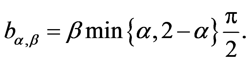
Considering a latent or an auxiliary variable, [1] proved a theorem that is useful to simulate samples of the joint posterior distribution for the parameters α, β, δ and σ. This theorem establishes that a stable distribution for a random variable Z defined in (−∞, ∞) is obtained as the marginal of a bivariate distribution for the random variable Z itself and an auxiliary random variable Y. This variable Y is defined in the interval (−0.5, a_α,β), when, and in (a_α,β, 0.5), when. The quantity a_α,β is given by

(1.3)

where

The joint probability density function for random variables Z and Y is given by

, (1.4)

where

(1.5)

and

, for

From the bivariate density (1.4), [1] shows the marginal distribution for the random variable Z is stable S_a (, 0, 1) distributed. Usually, the computational costs to obtain posterior summaries of interest using MCMC methods are high for this class of models, which could give some limitations for practical applications. One problem can be the simulation algorithm convergence. In this paper, we propose the use of a popular free available software to obtain the posterior summaries of interest: the OpenBUGS software.

The paper is organized as follows: in Section 2 we introduce a special case of the stable distributions, namely, the Lévy distribution. In Section 3, we introduce a Bayesian analysis for stable distributions. Two applications are presented in Section 4. Section 5 is devoted to some concluding remarks.

2. A Special Case of Stable Distributions: Lévy Distribution

Some special cases of stable distributions are given for specified values of α and β. If α = 2 and β = 0 one has the Gaussian distribution with δ mean and variance equals to If and one has a Lévy distribution with probability density function given by

(2.1)

for δ< x< ∞. Figure 1 presents Lévy probability density functions for δ = 0 and different values of the σ scale parameter.

The probability distribution function of the random variable X with a Lévy distribution defined in (2.1) is given by

(2.2)

where is the complementary error function with the error erf(.) given by

(2.3)

The Lévy distribution with probability density function (2.1) has undefined mean and undefined variance but its median is given by

, (2.4)

where the inverse complementary error function is

To obtain the probability, density function or the median of a random variable X with a Lévy density function different approximations for the complementary error function are introduced in the literature (see [13]). Some special cases are presented below.

1)

(2.5)

where the maximum error is 5 × 10⁻⁴ and a₁ = 0.278393, , and;

2)

(2.6)

where the maximum error is,

,

,

,

,

and

;

3)

, (2.7)

where

and sign(.) is given by (1.2).

4) An approximation for the inverse error function is given by

,(2.8)

where the constant a and the sign (.) are given in (2.7).

Assuming a random sample of size n with a Lévy distribution with probability density as (2.2), the likelihood function for δ and σ is given by

, (2.9)

where I (A) denotes the indicator function of set A.

Inferences for δ and σ parameters in the case of Lévy distribution are obtained using standard Markov Chain Monte Carlo methods (see [14,15]).

3. A Bayesian Analysis for General Stable Distributions

Let us assume that, for, is a random sample of size n, where, that is,

.

Assuming a joint prior distribution for α, β, δ and σ, given by, [1] shows that the joint posterior distribution for parameters and σ is given by

, (3.1)

where

, for, , , and; and are respectively, the observed and non-observed data vectors. Notice that the bivariate distribution in expression (3.1) is given in terms of and the latent variables, and not in terms of and (there is the Jacobian multiplied by the right-hand-side of expression (1.4)).

Observe that when α = 2 one has θ = 2 and. In this case one has a Gaussian distribution with δ mean and variance.

For a Bayesian analysis of the proposed model, we assume uniform U(a,b) independent priors for and, where the hyperparameters a and b are assumed to be known in each application following the restrictions, , and.

In the simulation algorithm to obtain a Gibbs sample for the random quantities and σ having the joint posterior distribution (3.1), we assume a uniform U(−0.5, 0.5) prior distribution for the latent random quantities for Observe that, in this case, we are assuming . With this choice of priors, one has the possibility to use standard software package like OpenBUGS (see [16]) with great simplification to obtain the simulated Gibbs samples for the joint posterior distribution.

In this way, one has the following algorithm:

1) Start with the initial values, , ,;

2) Simulate a sample from the conditional distributions, for;

3) Update, , , by, , , from the conditional distributions π, ,), , ,), , ,) and, ,);

4) Repeat Steps 1), 2) and 3) until convergence.

From expression (3.1), the joint posterior probability distribution for and is given by

(3.2)

where θ and are respectively defined in (1.4) and (1.5) and is a U(−0.5, 0.5) density function, for.

Since we are using the OpenBUGS software to simulate samples for the joint posterior distribution, we do not present here all full conditional distributions needed for the Gibbs sampling algorithm. This software only requires the data distribution and prior distributions of the interested random quantities. This gives great computational simplification for determining posterior summaries of interest as shown in the applications below.

4. Some Applications

4.1. Buckle’s Data

In Table 1, we have a data set introduced by [1]. This is the daily price return data of Abbey National shares in the period from July 31, 1991 to October 08, 1991.

In Figure 2(a), we present the histogram of the returns ρ(.) time series (given in Table 2) while in Figure 2(b) we have the Gaussian probability plot for the same data. From these figures, one observes that the Gaussian distribution does not fit well the data.

Assuming a Lévy distribution with probability density function given in (2.1) for a Bayesian analysis we consider the following prior distributions for δ and σ, δ ~ U(−1, −0.0271) and σ ~ U (0, 1), where U(a,b) denotes a uniform distribution on the interval (a, b). Observe that the minimum value for the ρ(.) data is given by −0.0271 and, that is, To simulate samples for the joint posterior distribution for and σ, using standard MCMC methods, we have used OpenBUGS software which only requires the log-likelihood function and prior distributions for model parameters. In Table 3, we present the posterior summaries of interest considering a burn-in-sample of size 5000 discarded to eliminate the initial value effect. After this burn-in-sample period we simulate another 200,000 Gibbs samples taking every 10-th sample. This gives a final sample of size 20,000 to be used for finding the posterior summaries of interest. Convergence of the Gibbs sample algorithm was verified by trace-plots of the simulated Gibbs samples. From OpenBUGS output we obtain a Deviance Information Criterium (DIC) value equals to −151.7. In Figure 2, (red line), we have the plot of the fitted Lévy density with δ = −0.0487 mean and σ = 0.0391 as the scale parameter and the histogram of the ρ (.) returns.

Assuming a general stable distribution, we present in Table 4 the posterior summaries of interest obtained using OpenBUGS software considering the following priors: α ~ U(1, 2), β ~ U(−1, 0), δ ~ U(−0.5, 0.5) and σ ~ U(0, 0.5). In the simulation procedure, we have used a burn-in-sample of size 10,000 and another 490,000 Gibbs samples taking every 100-th sample. This gives a final sample of size 4900 to be used for finding the posterior summaries of interest.

In Figure 3, we have the trace-plots of the simulated Gibbs samples. In Figure 2, we also have the plot of the fitted stable distribution with α = 1.653, β = −0.3455, δ = 0.00782 and σ = 0.001132. We observe good fit of the stable distribution (black line). The obtained DIC value is

equal to −70480. From this value we conclude that the data is better fitted by the general stable distribution in contrast to the Lévy distribution (since it has smaller DIC value).

4.2. Coding and Non-Coding Regions in DNA Sequences

Crato, et al. [2] introduce the length distribution of coding and non-coding regions for all Homo Sapiens chromosomes available from the European Bioinformatics Institute. In this way they consider a transformation of the genomes in numerical sequences. As an illustration, we have, respectively, in Tables 5 and 6, the data for coding and non-coding length sequences for H. Sapiens chromosomes transformed in a logarithm scale (sequence CM000275 extracted from Table 2, in [2]).

Figure 4 presents the histograms of the data given in Tables 5 and 6, assuming a logarithm transformation. From these plots, we observe that a Gaussian distribution could not be a reasonable model for fitting the data. Assuming a Lévy distribution with probability density function (2.1) for a Bayesian analysis we consider the following prior distributions for δ ~ U (−1000, 1.0986), where 1.0986 is the minimum of the observations in

REFERENCES

- D. J. Buckle, “Bayesian Inference for Stable Distributions,” Journal of the American Statistical Association, Vol. 90, No. 430, 1995, pp. 605-613. doi:10.1080/01621459.1995.10476553
- N. Crato, R. R. Linhares and S. R. C. Lopes, “α-stable Laws for Noncoding Regions in DNA Sequences,” Journal of Applied Statistics, Vol. 38, No. 2, 2011, pp. 267- 271. doi:10.1080/02664760903406447
- P. Lévy, “Théorie des Erreurs la loi de Gauss et les lois exceptionelles”, Bulletin de la Société Mathématique de France, Vol. 52, No. 1, 1924, pp. 49-85.
- E. Lukacs, “Characteristic Functions,” Hafner Publishing, New York, 1970.
- J. P. Nolan, “Stable Distributions—Models for Heavy Tailed Data,” Birkhäuser, Boston, 2009.
- B. V. Gnedenko and A. N. Kolmogorov, “Limit Distributions for Sums of Independent Random Variables,” Addison-Wesley, Massachusetts, 1968.
- A. V. Skorohod, “On a Theorem Concerning Stable Distributions,” In: Institute of Mathematical Statistics, Ed., Selected Translations in Mathematical Statistics and Probability, Vol. 1, 1961, pp.169-170.
- I. A. Ibragimov and K. E. Černin, “On the Unimodality of Stable Laws,” Teoriya Veroyatnostei i ee Primeneniya, Vol. 4, 1959, pp. 453-456.
- M. Kanter, “On the Unimodality of Stable Densities,” Annals of Probability, Vol. 4, No. 6, 1976, pp.1006-1008. doi:10.1214/aop/1176995944
- W. Feller, “An Introduction to Probability Theory and Its Applications,” Vol. II. John Wiley, New York, 1971.
- P. Damien, J. Wakefield and S. Walker, “Gibbs Sampling for Bayesian Non-Conjugate and Hierarchical Models by Using Auxiliary Variables,” Journal of the Royal Statistical Society, Series B, Vol. 61, No. 2, 1999, pp. 331-344. doi:10.1111/1467-9868.00179
- M. A. Tanner and W. H. Wong, “The Calculation of Posterior Distributions by Data Augmen-Tation,” Journal of American Statistical Association, Vol. 82, No. 398, 1987, pp. 528-550. doi:10.1080/01621459.1987.10478458
- M. Abramowitz and I. A. Stegun, “Handbook of Mathematical Functions with Formulas, Graphs, and Mathematical Tables,” National Bureau of Standards Applied Mathematics Series, Vol. 65, Dover Publications, Washington DC, 1964.
- S. Chib and E. Greenberger, “Understanding the Metropolis-Hastings Algorithm,” The American Statistician, Vol. 49, No. 4, 1995, pp. 327-335.
- C. P. Robert and G. Casella, “Monte Carlo Statistical Methods,” 2nd Edition, Springer-Verlag, New York, 2004. doi:10.1007/978-1-4757-4145-2
- D. J. Spiegelhalter, A. Thomas, N. G. Best and D. Lunn, “WinBUGS User’s Manual,” MRC Biostatistics Unit, Cambridge, 2003.
NOTES
*Corresponding author.