Open Journal of Statistics
Vol.1 No.3(2011), Article ID:8071,14 pages DOI:10.4236/ojs.2011.13022
Double Autocorrelation in Two Way Error Component Models
1Department of Economics, University of Cocody, Abidjan, Cote-d’Ivoire
2Resource Economics, West Virginia University, Morgantown, USA
3Division of Finance and Economics, West Virginia University, Morgantown, USA
E-mail: kern.kymn@mail.wvu.edu
Received September 15, 2011; revised October 16, 2011; revised October 30, 2011
Keywords: Two Way Random Effect Model, Double Autocorrelation, GLS, FGLS
Abstract
In this paper, we extend the works by [1-5] accounting for autocorrelation both in the time specific effect as well as the remainder error term. Several transformations are proposed to circumvent the double autocorrelation problem in some specific cases. Estimation procedures are then derived.
1. Introduction
Following the works of [6], the regression model with error components or variance components has become a popular method for dealing with panel data. A summary of the main features of the model, together with a discussion of some applications, is available in [7-10] among others.
However, relatively little is known about the two way error component models in the presence of double autocorrelation, i.e, autocorrelation in the time specific effect and in the remainder error term as well.
This paper extends the works by [2-5] on the one-way random effect model in the presence of serial autocorrelation, and by [1] on the single autocorrelation two-way approach. It investigates some potential transformations to circumvent the double autocorrelation issue, along with some estimation procedures. In particular, we derive several transformations when the two disturbances follow various structures: from autoregressive and moving-average processes of order 1 to a general case of double serial correlation. We deduce several GLS estimators as well as their asymptotic properties and provide a FGLS version.
The remainder of this paper is organized as follows: Section 2 considers simple transformations on the presence of relatively manageable double autocorrelation structure. In Section 3, general transformations are considered when the double autocorrelation is more complex. GLS estimators are derived in Section 4. Asymptotic properties of the GLS estimators are considered in Section 5. Section 6 provides a FGLS counterpart approach. Finally, some concluding remarks appear in Section 7.
2. Simple Transformations
To circumvent the double autocorrelation issue, we first need to transform the model based on the variance-covariance matrix. The general regression model considered is ,
, ;
;  where
where  is the intercept and
  is a
is a  vector of slope coefficients,
  is a
is a  row vector of explanatory variables which are uncorrelated with the usual two-way error components disturbances
 (see [7]). In matrix form, we write
 .
.
2.1. When the Errors Follow AR(1) Structures
If the time specific term follows an AR(1) structure,  ,
,  , with
 , and the remainder error term also follow an AR(1) structure
 ,
,  , with
 , we can define two transformation matrices of dimensions
  and
and  respectively,

 (1)
(1)
and since we have

and
 (2)
(2)
the transformed errors  and
and  follow two different MA(1) processes, of parameters
  and
and  respectively. Thus, by applying the appropriate transformation matrices, the autoregressive error structure can be changed into a moving-average one. The only cost is the loss of the initial and first pseudo-differences, which has no serious consequence for a long time dimension. As a result, we focus on the MA(1) error structure.
2.2. When the Errors Follow MA(1) Structures
Here, the time specific term  follows an MA(1) structure,
 ,
,  with
with  while the remainder error term,
  also follows an MA (1) structure,
  ,
,  with
with  . For convergence purpose and assuming normality, the initial values are defined

and

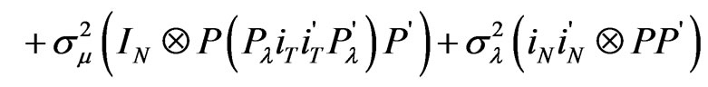
The variance-covariance matrix of the three components error term is given by,
 (3)
(3)
where  and
and  are positive definite matrices of order
  and where
  is defined by
 . The exact inverse of such matrices suggested by [11] and [1] does not involve the parameters
  and
and . Following [11], let
  be the Pesaran orthogonal matrix whose t-th row is given by,

where
 ,
,  ,
,  ,
,  and
and  with
with .
.
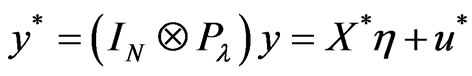
Pre-multiplying the model by  yields the following variance-covariance matrix of
 ,
,
 (4)
(4)
where .
.
3. General Transformations
We are now in the context of a general case of double autocorrelation issue and lead to a suitable error covariance matrix similar to Equation (4) and its inverse.
3.1. First Transformation
Let  denote the matrix such that
 . Such a matrix does exist for
  and is a positive-definite matrix. Transformation of the initial model
 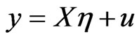 by
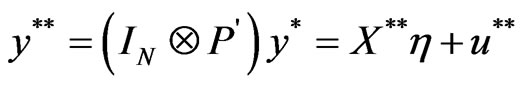
by  yields
 (5)
(5)
and the variance-covariance of the transformed errors is
 (6)
(6)
This transformation has removed the autocorrelation in the time-specific effect . Unfortunately, by doing so it has infected the
  and worsened the initial correlation in the remainder disturbances. An additional “treatment” is therefore needed.
3.2. Second Transformation
We now consider an orthogonal matrix  and a diagonal matrix
  such that
  (diagonalization of
 ). Thus, applying a second transformation
  yields,
 (7)
(7)
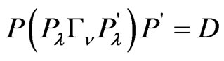
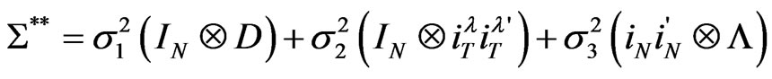
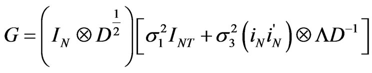
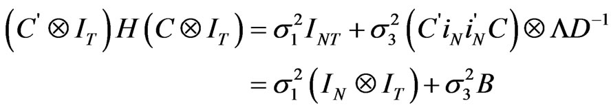
The underlying variance-covariance matrix of the errors is,

 (8a)
(8a)
or,
 (8b)
(8b)
where ,
,  ,
,  ,
,  ,
,  , and
, and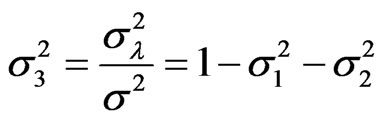 , if
, if .
.
Here, because of the choice of matrices  and
and , we end up with
  since
since  is an orthogonal matrix. Generally speaking,
  and
and  just need to have zero off-diagonal elements, i.e., to be diagonal matrices. The double autocorrelation structure is thus absorbed, and one can easily accommodate with the non-spherical form of
  by means of an accurate inversion process.
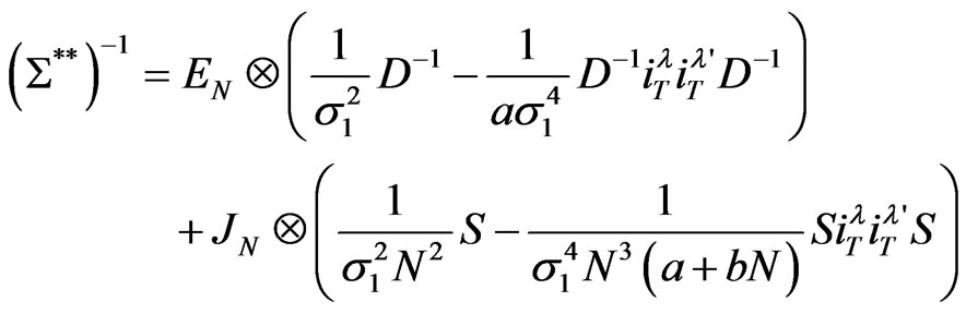
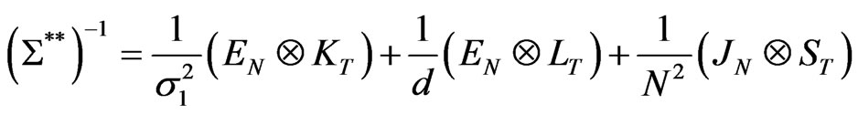
3.3. Computing the Inverse
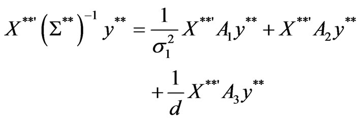
The inverse of  is obtained using the procedure developed by [1]. After a bit of algebra, one gets
 (9)
(9)
where
 ,
,  ,
,  ,
,  ,
,  ,
, 
and
 with
with .
.
Proof: (see the Appendix)
4. GLS Estimation
We begin with the definition of the estimator followed by its interpretation and weighted average property.
4.1. The GLS Estimator
Proposition 1:
The GLS estimator is,
 (10)
(10)
Proof: (Straightforward)
4.2. Interpretation
In classical two-way regression models, [12,13] provide an interpretation of the GLS estimator, which is appealing in view of the sources of variation in sample data. In the straight line of their work, the GLS estimator may be viewed as obtained by pooling three uncorrelated estimators: the covariance estimator (or within estimator), the between-individual estimator and the within-individual estimator. They are the same as those suggested by [1] except for the last one which was labeled between-time estimator. We have
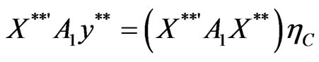
1) The covariance estimator,
 where
where ;
;
2) The between-individual estimator,
 where
where  and
and
3) The within-individual estimator,
 where
where .
.
It is important to note that these estimators are obtained from some transformations of the regression Equation (7), i.e.,
 .
.
The covariance estimator,  is obtained when Equation (7) is pre-multiplied by
 ; the transformation annihilates the individualand time-effects as well as the column of ones in the matrix of explanatory variables. It is equivalent to the within estimator in the classical two-way error component model (see [1-7]).
The between-individual estimator  comes from the transformation of Equation (7) by the matrix
  . This is equivalent to averaging individual equations for each time period.
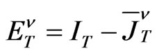
The within-individual estimator  is derived when Equation (7) is transformed by
 . The presence of the idempotent matrix
  indicates that this transformation wipes out the constant term as well as the time specific error term
 . However, the individual effect
  remains.
4.3. GLS as a Weighted Average Estimator
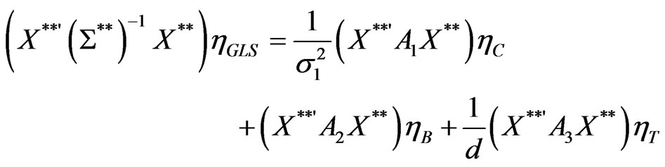
As in [14], the GLS estimator is a weighted average of the three estimators defined above.
Proposition 2:
 (11)
(11)
with,
 ,
,  and
and

Proof:
From Equation (10), it comes that

with
By definition, the estimators ,
,  and
and  are respectively such that
 ,
,
 and
and
 .
.
Therefore,

Or,
Thus,

with ,
,  and
and  defined according to Equation (11).
We should also note that the three estimators ,
,  and
and  are uncorrelated. In fact,

and
because , while
  since
since  . As a result,
 (12)
(12)
Moreover, following [1], the fact that
 (13)
(13)
gives evidence on the use of all available information from the sample. The estimators ,
,  and
and  together use up the entire set of information to build the GLS estimator
  with no loss at all.
5. Asymptotic Properties
Under regular assumptions, the GLS and the three pseudo estimators of the coefficient vector, say ,
,  ,
,  and
and  are all consistent and asymptotically equivalent. It is a result similar to the one obtained in the classical two-way error component model (see [15]).
5.1. Assumptions
We assume that the  are weakly non-stochastic, i.e. do not repeat in repeated samples. We also state that the following matrices exist and are positive definite:

for the first transformation;
for the second transformation; and
for the third transformation. Furthermore, in the straight line of [1], we also assume that,

for the first transformation;

for the second transformation;

for the third transformation. In addition,
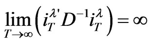 , so that the variance-components quantity
  denotes by
  remains infinite as
 . The limits and probabilities are taken as
  and
and . All along this section, following [1], we consider the “usual” assumptions regarding the error vector
 , as stated in [16] and [17], which ensures the asymptotic normality.
5.2. Asymptotic Property of the Covariance Estimator
Proposition 3:
The covariance estimator  is consistent.
Proof:
Since,

Hence,
Making use of assumptions (a1) and (a2), we establish the consistency of the covariance estimator, .
.
Proposition 4:
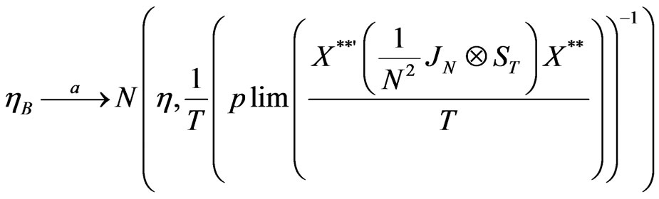
The covariance estimator  has an asymptotic normal distribution given by,
 (14)
(14)
Proof:
Under the M1-transformation, we have
 .
.
Moreover its variance is given by 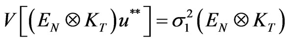 and its inverse is equal to
  while assumption (a2) states the absence of correlation between regressors and disturbances under the M1 transformation. We have
 (15)
(15)
and,

from which we deduce that
 .
.
Thus, the asymptotic normality of the covariance estimator immediately follows,
 .
.
5.3. Asymptotic Property of the Between-Time Estimator
Proposition 5:
The between time estimator  is consistent.
Proof:
Since,

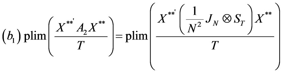
Hence, according to assumptions (b1) and (b2),

Making use of assumptions (b1) and (b2), we establish the consistency of the between time estimator,
 .
.
Proposition 6:
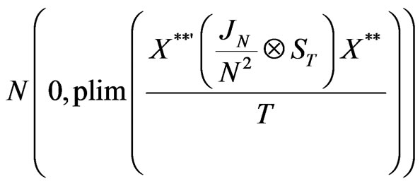
The between-time estimator  has an asymptotic normal distribution given by,
 (16)
(16)
Proof:
Under the M2-transformation, we get

The variance of this error term is written as

Its inverse is . Again, assumption (b2) states the absence of correlation between regressors and disturbances under the M2 transformation. We get

In addition, we have

from which we deduce that

Thus, the asymptotic normality of the between-time estimator immediately follows,
 .
.
5.4. Asymptotic Property of the Within-Individual Estimator
Proposition 7:
The within individual estimator  is a consistent estimator.
Proof:
Since,

Hence,

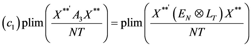
Making use of assumptions (c1) and (c2), we establish the consistency of the covariance estimator,

Proposition 8:
The within individual estimator  has an asymptotic normal distribution given by,
 (17)
(17)
Proof:
Under the M3-transformation, we obtain

The variance of  is obtained as

The inverse of this matrix is . Assumption (c2) states the absence of correlation between regressors and disturbances under the M3 transformation. We have

and,

from which we deduce that

Thus, the asymptotic normality of the within individual estimator immediately follows,

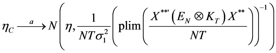
5.5. Asymptotic Property of the GLS Estimator
Proposition 9:
The GLS estimator  is asymptotically equivalent to the covariance estimator
  and therefore,
 (18)
(18)
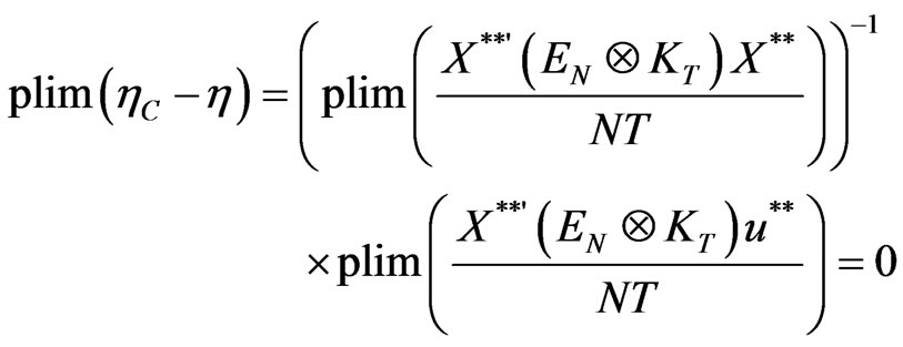
Proof:
From Equation (10), we get

On the one hand, we have

where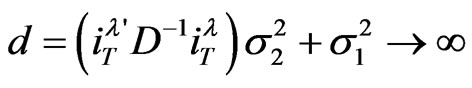 , as
, as . Therefore, from assumption (a1), we find that
  , when
 . Likewise, assumption (a2) leads us to
 , when
 . Hence,

On the other hand, we can write
 .
.
Under the M1 and M2 transformations, we get

leading to
 .
.
As a result,

i.e.,

Finally,  has the same limiting distribution as
 . This shows the asymptotic equivalence of the two estimators
  and
and . We then deduce that,

Thus, the GLS estimator suggested under the double autocorrelation error structure has the desired asymptotic properties.
6. FGLS Estimation
In practice, the variance-covariance matrix is unknown, as well as all the parameters involved in its determination. Therefore, a FGLS approach is required. The method used consists in removing the time specific effect to obtain a one-way error component model where only  carries the serial correlation (see [18] and [3]). This method has been directly applied to AR(1) and MA(1) processes in separate subsections.
6.1. Feasible Double AR(1) Model
We assume that ,
,  ,
,  ,
,  ,
,  ,
, . The within error term is,
 (19)
(19)
The associated variance-covariance matrix is,
 (20)
(20)
Since  follows an AR(1) process of parameter
 , we define the matrix
  as the familiar [19] transformation matrix with parameter
 . This matrix is such that,

The resulting GLS estimator is given by
 (21)
(21)
where 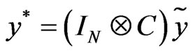 and
and .
.
The covariance matrix of , using [20] trick, is
 (22)
(22)
where

 ,
, 
and

Following [21], another GLS estimator can be derived. We label this estimator the within-type estimator and is given by
 (23)
(23)
with  and
and . In order to get the estimates of numerous parameters involved in the model, we first need an estimate of the correlation coefficient
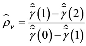
 . The autocorrelation function of the error term
  is given by
 (24)
(24)
We deduce from it that . It then leads to a convergent estimator of
  (see [7]), i.e.,
where  with
with  defined as the OLS residuals of the within equation
 . Hence, we get
 (25a)
(25a)
and
 (25b)
(25b)
Furthermore, the BQU estimate of  is also available as
 (26)
(26)
 being the OLS estimate of
 . As a consequence, we get
 (27a)
(27a)
and
 (27b)
(27b)
We now need to find  and
and . The autocovariance function of the initial error term
  is given

for .
.
It comes that,
 (28)
(28)
We immediately deduce a convergent estimator of the second correlation coefficient, i.e.,
 (29)
(29)
where  with
with  denoting the OLS residuals of
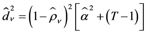
 . The variances
  is estimated by,
 (30)
(30)
In addition to the GLS estimators mentioned in Section 4, other GLS estimators such as the within estimator  and the within-type estimator
  can all be performed as well. Actually, the knowledge of the AR(1) parameters
  and
and  entitles us to build the matrices involved in the determination of
 , say matrices
 ,
,  ,
,  ,
,  ,
,  ,
,  ,
,  ,
,  ,
,  and
and .
.
6.2. Feasible Double MA(1) Model
We now state that , with
  and
and . Again, deviations from individual means lead to the model
 with
with .
.
The variance-covariance matrix of  is still given by Equation (20), with now
 (31)
(31)
Here, we set ,
,  denoting the correlation correction matrix as defined by [8] in their orthogonalizing algorithm. We then transform the within model by
 . The new error term
  has the following covariance matrix,
 (32)
(32)
Because of the moving average nature of the process, linear estimation of the correlation parameter  is not easily obtainable. Instead,
  proves useful. The autocorrelation function of the within error term
  is given by,
 (33)
(33)
with  denoting the autocovariance function of
 . As a consequence,
  for some
 and
and
 (34)
(34)
where  is the empirical autocovariance function and
  are the OLS residuals of the within equation. We also get, for some
 ,
,
 (35)
(35)
We then apply the [8] matrix  to the data (for instance to the within transformed dependent vector
 ). Moreover,
  will be applied to the vector of constants to get estimates of the
 . We have, in the straight line of [8], the following steps:
Step 1: Compute  and
and
 for
for 
where  for
for .
.
Step 2: Compute  knowing that
 . The estimates of the
  are obtained as
  and
and
 for
for .
.
We then obtain the estimate of  as
as . The autocovariance function
  of the initial composite error term
  and its empirical counterpart
 , (
, ( being the OLS residuals of the initial two-way model) permit the estimation of
  and
and ,
,
 (36a)
(36a)
and
 (36b)
(36b)
The within estimator  and the within-type one
  are now obtainable. However, the GLS estimator
  can be estimated, provided the MA(1) parameters
  and
and  are known, especially under the conditions
 and
and . In other words, the estimates
  and
and  should both lie inside the open interval
  as a pre-requisite to a direct estimation of
 ,
,  ,
,  and
and .
.
7. Final Remarks
This paper has considered a complex but realistic correlation structure in the two-way error component model: the double autocorrelation case. It dealt with some parsimonious models, especially the AR(1) and MA(1) ones, as well as the general framework. Through a precise formula of the variance-covariance matrix of the errors, we derived the GLS estimator and related asymptotic properties. An investigation of the FGLS is also considered in the paper.
8. References
[1] N. S. Revankar, “Error Component Models with Serial Correlated Time Effects,” Journal of the Indian Statistical Association, Vol. 17, 1979, pp. 137-160.
[2] B. H. Baltagi and Q. Li, “A Transformation that will Circumvent the Problem of Autocorrelation in an Error Component Model,” Journal of Econometric, Vol. 48, No. 3, 1991, pp. 385-393. doi:10.1016/0304-4076(91)90070-T
[3] B. H. Baltagi and Q. Li, “Prediction in the One-Way Error Component Model with Serial Correlation,” Journal of Forecasting, Vol. 11, No. 6, 1992, pp. 561-567. doi:10.1002/for.3980110605
[4] B. H. Baltagi and Q. Li, “Estimating Error Component Models with General MA(q) Disturbances,” Econometric Theory, Vol. 10, No. 2, 1994, pp. 396-408. doi:10.1017/S026646660000846X
[5] J. W. Galbraith and V. Zinde-Walsh, “Transforming the Error Component Model for Estimation with general ARMA Disturbances,” Journal of Econometrics, Vol. 66, No. 1-2, 1995, pp. 349-355. doi:10.1016/0304-4076(94)01621-6
[6] P. Balestra and M. Nerlove, “Pooling Cross-Section and Time-Series Data in the Estimation of a Dynamic Model: The Demand for Natural Gas,” Econometrica, Vol. 34, No. 3, 1966, pp. 585-612. doi:10.2307/1909771
[7] B. H. Baltagi, “Econometric Analysis of Panel Data,” 3rd Edition, John Wiley and Sons, New York, 2008.
[8] C. Hsiao, “Analysis of Panel Data,” Cambridge University Press, Cambridge, 2003.
[9] G. S. Maddala, “Limited Dependent and Qualitative Variables in Econometrics,” Cambridge University Press, Cambridge, 1983.
[10] G. S. Maddala, “The Econometrics of Panel Data,” Vols I and II, Edward Elgar Publishing, Cheltenham, 1983.
[11] M. H. Pesaran, “Exact Maximum Likelihood Estimation of a Regression Equation with a First Order Moving Average Errors,” The Review of Economic Studies, Vol. 40, No. 4, 1973, pp. 529-538.
[12] P. A. V. B. Swamy and S. S. Arora, “The Exact Finite Sample Properties of the Estimators of Coefficients in the Error Components Regression Models,” Econometrica, Vol. 40, No. 2, 1972, pp. 261-275. doi:10.2307/1909405
[13] M. Nerlove, “A Note on Error Components Models,” Econometrica, Vol. 39, No. 2, 1971, pp. 383-396. doi:10.2307/1913351
[14] G. S. Maddala, “The Use of Variance Components Models in Pooling Cross Section and Time Series Data,” Econometrica, Vol. 39, No. 2, 1971, pp. 341-358. doi:10.2307/1913349
[15] T. Amemiya, “The Estimation of the Variances in a Variance-Components Model,” International Economic Review, Vol. 12, No. 1, 1971, pp. 1-13. doi:10.2307/2525492
[16] H. Theil, “Principles of Econometrics,” John Wiley and Sons, New York, 1971.
[17] T. D. Wallace and A. Hussain, “The Use of Error Components Models in Combining Cross-Section and Time Series Data,” Econometrica, Vol. 37, No. 1, 1969, pp. 55- 72. doi:10.2307/1909205
[18] T. A. MaCurdy, “The Use of Time Series Processes to Model the Error Structure of Earnings in a Longitudinal Data Analysis,” Journal of Econometrics, Vol. 18, No. 1, 1982, pp. 83-114. doi:10.1016/0304-4076(82)90096-3
[19] S. J. Prais and C. B. Winsten, “Trend Estimators and Serial Correlation,” Unpublished Cowles Commission Discussion Paper: Stat No. 383, Chicago, 1954.
[20] W. A. Fuller and G. E. Battese, “Estimation of Linear Models with Cross-Error Structure,” Journal of Econometrics, Vol. 2, No. 1, 1974, pp. 67-78. doi:10.1016/0304-4076(74)90030-X
[21] T. J. Wansbeek and A. Kapteyn, “A Simple Way to obtain the Spectral Decomposition of Variance Components Models for Balanced Data,” Communications in Statistics, Vol. 11, No. 18, 1982, pp. 2105-2112.
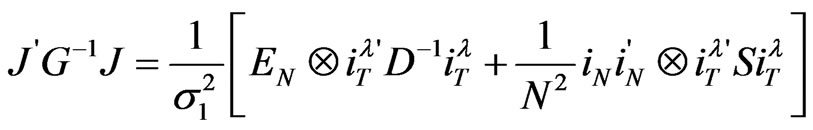
Appendix: Computing the Inverse of 
We established that
with  and
and .
.
Setting , we can rewrite the variance covariance matrix as

where . By the means of an update formula, we deduce an expression of the inverse of
 ,
,

We need to obtain  and the inverse of the bracketed expression. On the one hand,

Let  denote the matrix
 . At this step, the inverse of
  is required. Let
  be a
be a  orthogonal matrix. Then,
Therefore,

with
 .
.
It is worth mentioning that  for
for  and
and  are different columns of the same diagonal matrix. It is therefore obvious that
  has already been diagonalized. As a consequence, the inverse of
  is given by,


where

Since  and
and , we have
 .
.
Therefore,

It then follows that,


in which  with
with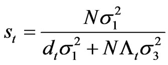 ,
, .
.
On the other hand, the matrix  has to be determined. We get,

or,
Thus,

Hence,

and,

where
 and
and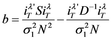 .
.
Since
 we deduce
 .
.
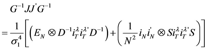
We are now interested in the expression
 .
.
We have,
From the definitions of the matrices  and
and , we can write
 and
and
 so that
and lastly

It then comes that

In other words,

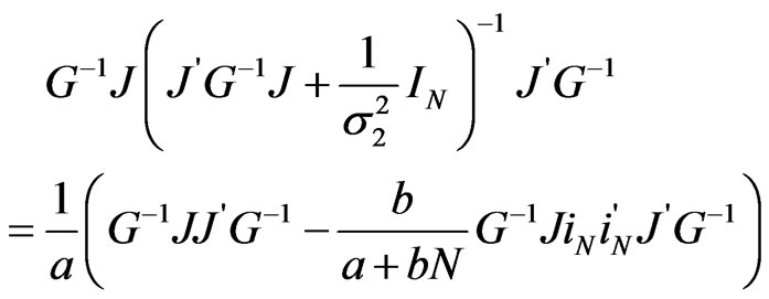
Finally, the inverse of  can be derived as
with . An alternative expression for
  is available. Setting
 , and
, and
 , we get


where

i.e.,

Hence, we finally get
where 