Journal of Mathematical Finance Vol.05 No.01(2015), Article ID:54073,14
pages
10.4236/jmf.2015.51006
Interest Rate Volatility: A Consol Rate Approach
Vincent Brousseau1, Alain Durré2*
1Visiting Scholar at Lille 2-Skema Management Research Center-Centre National de la Recherche Scientifique (E.A. 4112), Lille, France 2IéSEG-School of Management (Lille Catholic University) and LEM-Centre National de la Recherche Scientifique (U.M.R. 8179), Paris, France
Email: vincent.brousseau@univ-lille2.fr, *a.durre@ieseg.fr
Copyright © 2015 by authors and Scientific Research Publishing Inc.
This work is licensed under the Creative Commons Attribution International License (CC BY).
http://creativecommons.org/licenses/by/4.0/


Received 22 January 2015; accepted 10 February 2015; published 13 February 2015
ABSTRACT
In this paper, we propose a new methodology to estimate the volatility of interest rates in the euro area money market. In particular, our approach aims at avoiding the limitations of market implied volatilities, i.e. the dependency on arbitrary choices in terms of maturity and frequencies and/or of other factors like credit and liquidity risks. The measure is constructed as the implied instantaneous volatility of a consol bond that would be priced on the EONIA swap curve over the sample period from 4 January 1999 to 21 November 2013. Our findings show that this measure tracks well the historical volatility since, by dividing the consol excess returns by our volatility measure. This removes nearly entirely excess of kurtosis and volatility clustering, bringing the excess returns close to an ordinary Gaussian white noise.
Keywords:
Consol Rate, Historical Volatility, Overnight Money Market, Interbank Offered Interest Rates

1. Introduction
It is common that the logarithm of asset prices is not well depicted by a simple Brownian motion. The first feature of a Brownian motion, which is a Gaussian white noise, is the absence of excess of kurtosis, and the square or the absolute value of this first difference exhibits no autocorrelation. By contrast, the returns of an asset exhibit noticeable excess of kurtosis, and their square or their absolute returns exhibit positive autocorrelations. Attempts to find a better modelling for the log-prices may include the adjunction of jumps or the specification of a variable, generally random, volatility. A variable volatility is sufficient to produce the excess of kurtosis and the positive autocorrelation of squared and absolute values―known as “volatility clustering”. Therefore, it is legitimate to wonder whether the recourse to variable volatilities is sufficient to capture the observed features of kurtosis excess and volatility clustering.
To answer this question, one may start with the following thought experiment. Consider the observed time series of a liquidly traded asset price, for instance the euro-dollar exchange rate. Ignoring the short-term interest rates that prevail on those two currencies, we assume for simplicity that two subsequent observations are never identical. The corresponding return is thus the difference of the log-price at time t + 1 and at time t. Then, we define the proxy of its instantaneous volatility, at time t, by the absolute value of that return. The normalised return is therefore defined as the ratio of the return and of that proxy. By construction, this normalized return is a random sequence of +1 and −1. It will exhibit no autocorrelation, and its distribution will be even less leptokurtic than a Gaussian one, which means that it has a negative excess of kurtosis. This can be the basis of a procedure for constructing the instantaneous volatility of the exchange rate, if and only if the value of that rate at time t + 1 is known at time t, which is obviously not the case. So one is led to reformulate the initial question as follows: is it possible to construct a proxy of the instantaneous volatility at time t with data available at time t, in such a way that the return normalized by this proxy exhibits neither excess of kurtosis nor autocorrelation of its square or of its absolute value?
Here, there are two possible ways forward. One might construct that proxy on the basis of the history of the series available at time t, or, on the other hand, one might take recourse to exogenous data available at time t, namely the corresponding market-implied volatilities. The second way should be favoured because it does not assume anything about the statistical properties of the price series. In the example of the euro-dollar exchange rate, the exercise could be described by the following steps: a) to reconstruct an instantaneous volatility from the available market implied volatilities; b) to calculate the excess return of the exchange rate taking into account short-term interest rates of the two currencies; c) to calculate the normalised excess return by dividing the excess return by the instantaneous volatility; and d) to compare the statistical properties of the raw excess returns and of the normalised one. If the raw excess returns exhibit excess of kurtosis and volatility clustering whereas the normalised retruns do not, then it means that it is possible to model the exchange rate as an Ito process with variable volatility.
This paper follows the same approach with an application to the money market yield curve. The case of the yield curve is substantially more complex than the case of the exchange rate since it has a structure in contrast with a single interest rate which is reduced to a number. Furthermore, it is impossible to ignore the short-term interest rate in the case of the yield curve as it is a constitutive element of the curve under study. Finally, there is not one traded asset that could be representative of the yield curve.
The contribution of our analysis to the literature is to suggest a simple way to circumvent the above-men- tioned technical difficulties. In particular, it uses as the representative asset a perpetuity paying a constant rate of dividend, called the consol rent, priced from the curve. It defines its excess return, constructs an instantaneous volatility from market-implied ones, constructs the corresponding normalised excess return and compares the statistical features of raw and normalized excess returns. Our results show that the consol rate can be described as an Ito process with variable volatility, hence avoiding the inclusion of jumps.
The paper is organised as follows. After this introduction, Section 2 summarizes the purpose and the main steps of our approach before Section 3 presents the useful definitions of key parameters, namely the consol excess return, the consol volatility and the consol normalized excess returns. Section 4 then compares the statistical features of consol excess return and consol normalized excess return when the process of the curve is simulated according to two arbitrage-free theoretical models. Section 5 compares the statistical features of consol excess return and consol normalized excess return for the EONIA swap curve. Finally, Section 6 concludes while the reconstruction of the consol normalized excess returns and volatility for that empirical EONIA swap curve is described in the annex.
2. Presentation of the Exercise
The proposed exercise requires two preliminary steps: first, an accurate definition of the excess return relevant for the consol rate; second, a construction of the consol rate, excess return and volatility. Then, a comparison between the excess return and the normalized excess return of excess of kurtosis and of ACF of squared and absolute values for an empirical yield curve will allow to evaluate the quality of the measure. The empirical yield curve chosen in the paper is the one implied by the EONIA swaps, which is considered as the riskless curve for the euro currency.
The central idea is to claim that if some computed volatility does lead to normalized excess returns free of excess of kurtosis and of autocorrelation in squared and absolute values, then it can be regarded as the volatility of the consol rent1. In order to support the previous conclusion, it is therefore useful to see what happens in cases where the true volatility is effectively known. It is effectively known in the case of some arbitrage-free yield curve models. So a way to judge the validity of the proposed criterion is to apply it in the case of simulated trajectories of the yield curve, when the simulation follows an arbitrage-free model for which the volatility can be effectively computed, and for which the length of the sample is the same as the length of the available sample of empirical data.
3. Consol Rate, Consol Excess Return, Consol Volatility
Let us first recall some key mathematical notions related to the concepts of yield curve and of consol rate, before discussing the basic properties of a consol volatility. From those basic properties, it follows that the consol volatility reduces the consol excess returns to a Gaussian white noise, within the mathematical frameworkof a continuous-time arbitrage-free model. This hints that, in the real world, a correct measure of volatility should also be able to reduce the excess returns to a Gaussian white noise. This can be tested by examining whether dividing the excess returns by the volatility actually reduces the leptokurticity and the volatility clustering. This test will be illustrated with simulated data, for which the true volatility can be known ex ante, before being presented for the actual euro data. In this case, a success of the test indictes that the true volatility can be, and has effectively been, recovered.
3.1. Notational Convention
The purpose of this paragraph is to recall and define the key notions of this paper within the continuous-time framework, as well as their basic mathematical properties. For convenience, the following convention is adopted: Latin letters denote dates while Greek letters refer to delay/duration between two dates2.
3.1.1. Zero-Coupon and Forward Rates
Yield curves are formally defined as functions of a continuous time parameter, which
associate an interest rate to a maturity within a (theoretically unbounded) maturity
set. Yield curves are also usually expressed in mainly two ways: a) as zero-coupon
interest rate curves; or b) as instantaneous forward interest rate curves. These
two ways are equivalent and convey the same quantity of information. With
 the zero-coupon interest rate at maturity
 ,
,
 the forward
interest rate at maturity
the forward
interest rate at maturity
 (whereby both interest rates are continuously com- pounded) and
 the spot price of the zero coupon of maturity
 , i.e. the present value of one currency unit to be paid over
 , one can write that:
 (1)
(1)
and
 (2)
(2)
which implies the following mathematical relationship between zero-coupon interest rate and the forward in- terest rate:
 (3)
(3)
or, conversely, as the change of variables is duly invertible:
 (4)
(4)
From Equations (3) and (4), it follows two basic but important properties follow:
a)
 is constant
if and only if
is constant
if and only if
 is constant. In this particular case, it means that the constant value taken by
 is the same as the constant value taken by
 ,
which would imply a flat yield curve while the constant value taken by both
,
which would imply a flat yield curve while the constant value taken by both
 and
and
 is called the level of the flat yield curve;
b) irrespective of the shape of the yield curve,
 and
and
 are always equal and the corresponding unique value defines the short-term interest
rate
are always equal and the corresponding unique value defines the short-term interest
rate ,
i.e.
,
i.e. .
.
Note also that one defines as parallel shift in the remainder of the analysis a transformation of the yield curve such as a constant is added to the zero-coupon interest rates, or, equivalently, of the forward rates following from Equation (3).
3.1.2. Consol Bond and Consol Rate
A consol bond is defined as a perpetual (infinite horizon) bond paying continuously a constant rate of money, which is called the coupon flow. By definition, the consol price C is defined as the price of the consol bond divided by the coupon flow3, which can be expressed, in terms of the yield curve, as follows:
 (5)
(5)
By substituting
 by its value using Equation (1), the consol price becomes:
 (6)
(6)
The consol rate,
 ,
defined as the yield of the consol bond, is the inverse value of the consol price,
i.e.4:
,
defined as the yield of the consol bond, is the inverse value of the consol price,
i.e.4:
 (7)
(7)
The consol duration,
 ,
that is the duration (in the sense of [2] ) of the consol bond reflecting the sensitivity
of the logarithm of the consol price to a parallel shift of the consol yield curve,
can be expressed as:
,
that is the duration (in the sense of [2] ) of the consol bond reflecting the sensitivity
of the logarithm of the consol price to a parallel shift of the consol yield curve,
can be expressed as:
 (8)
(8)
where the sensitivity of the consol rate to a parallel shift of the yield curve,
 ,
is given by the following product:
,
is given by the following product:
 (9)
(9)
This dimensionless number
 is equal to 1 in case of a flat curve. Empirical evidence shows that yield curves
have usually
is equal to 1 in case of a flat curve. Empirical evidence shows that yield curves
have usually
 smaller than, but close to, 1. We say that that a financial price is in constant
terms, by opposition to current terms, when it is expressed in currency values of
a fixed reference date in the past rather than in currency values of the current
date.
smaller than, but close to, 1. We say that that a financial price is in constant
terms, by opposition to current terms, when it is expressed in currency values of
a fixed reference date in the past rather than in currency values of the current
date.
Finally, the consol wealth process, denoted
 hereafter, is defined as the wealth, expressed in constant terms, of an ideal investor
facing no transaction costs or short-selling restrictions who holds a portfolio
of consol bonds in which he reinvests automatically the whole coupon flow at the
prevailing market price. Therefore, the corresponding (infinitesimal) consol excess
return, denoted
hereafter, is defined as the wealth, expressed in constant terms, of an ideal investor
facing no transaction costs or short-selling restrictions who holds a portfolio
of consol bonds in which he reinvests automatically the whole coupon flow at the
prevailing market price. Therefore, the corresponding (infinitesimal) consol excess
return, denoted ,
is written:
,
is written:
 (10)
(10)
whereby the first two terms refer to the nominal gain (or loss) due respectively
to the change in the market price of the consol bond
 and to the coupon flow
 while the third term
 refers to the carry cost of the position, i.e. holding the portfolio of consol bonds.
3.1.3. Volatility of a Consol Bond
The quadratic variation of a process
 is denoted
 ,
so that Ito’s formula is:
,
so that Ito’s formula is:
 (11)
(11)
The volatility of the consol bond,
 ,
is defined as:
,
is defined as:
 (12)
(12)
The differential
 (with
(with
 denoting the logarithm of the consol wealth process, hereafter referenced as to
consol performance) can be obtained by applying the Ito’s iteration to Equation
(10), i.e.:
denoting the logarithm of the consol wealth process, hereafter referenced as to
consol performance) can be obtained by applying the Ito’s iteration to Equation
(10), i.e.:
 (13)
(13)
which leads to the following identity using the Ito’s formula:
 (14)
(14)
Substituting Equation (14) into Equation (13) leads to express the consol excess return as:
 (15)
(15)
which, by applying Ito’s iteration to Equation (15), yields:
 (16)
(16)
Finally, the normalized excess return is defined as:
 (17)
(17)
which, by combining Equations (15), (16) and (17), yields:
 (18)
(18)
We will then apply the mathematical specification of the consol rate, and the calculation of the corresponding volatility as discussed from Equations (11) to (18), to standardise the volatility measure for interest rates in the money market.
3.1.4. Risk-Neutral Probability
Within the framework of Heath-Jarrow-Morton [3] , the dynamics of ,
,
 and
and
 are fully specified by the stochastic process of
 under risk-neutral probability.
 must
be a martingale, so Equations (10) and (12) imply:
must
be a martingale, so Equations (10) and (12) imply:
 (19)
(19)
with
 denoting a Wiener process, from which it immediately follows that:
 (20)
(20)
By combining Equations (15) and (19) under the risk-neutral probability, the change
of the yield of the consol, bond,
 ,
becomes:
,
becomes:
 (21)
(21)
By combining Equations (12), (15), (17) and (21), it follows:
 (22)
(22)
where
 itself is also a Wiener process under risk-neutral probability. This implies that:
 (23)
(23)
Equation (23) is valid not only under risk-neutral probability but also under any equivalent probability to the risk neutral probability, as it pertains to the quadratic variation only. Finally, Equations (18) and (22) yield that:
 (24)
(24)
Note the left-hand side of Equation (24) is defined as the normalized excess return.
It follows from Equation (24) that the the normalized excess returns―i.e. the excess returns divided by the true volatility―should be akin a Gaussian white noise under risk-neutral probability. As we know, empirical excess returns of any financial asset usually differ from a Gaussian white noise by two properties: a) their empirical distribution more kurtosis than the Gaussian distribution (the property of leptokurticity); and b) their absolute values (or their square values) have a positive serial correlation (the property of volatility clustering). To the extent that the Ito-process modelisation is a realistic representation of the consol rate dynamics, one should be able to remove those two properties, by dividing the excess returns by a correct measure of the underlying volatility, and that operation of normalization would recover the underlying Gaussian white noise process.
4. Data
The dataset contains only TARGET working days; it contains all the TARGET working days from 4 January 1999 to 21 November 2013, which represents 3816 TARGET working days. The financial instruments taken into account are handled in the OTC market. They consist into: short-term unsecured deposit of maturity 1-day (overnight, tom-next and spot-next), EONIA swaps from 1-week to 30-year, 6-month EURIBOR swaps for the corresponding maturities, at-the-money implied volatilities of options on the EURIBOR swaps.
We used the options on 6-month EURIBOR swaps with option maturity 1-month, 3-month, 6-month, 1-year, 2-year, 3-year, 4-year and 5-year, and with underlying EURIBOR swap maturity 1-year, 2-year, 3-year, 4-year, 5-year, 7-year, 10-year, 15-year, 20-year, 25-year and 30-year. Other maturities of options or of underlying swaps are represented in the quotes contributed by brokers, but their history may start at relatively recent dates, which makes preferable not to use them. Besides, the EONIA fixing is included in the dataset. Each instrument or fixing is identified in the Reuters database by a unique RIC (Reuters Instrument Code).
As the financial instruments taken into account are handled on the OTC market, we made use of quoted data, generally given as a bid-ask spread from which we retained only the mid. We gave a preference to quotes issued by the broker ICAP, and when not available, our primary fallback was the generic quote of Reuters, which contains the latest quote issued by a bank or broker at the time of its snapshot or of its contribution. In case of missing data, the data set is completed by a reconstruction of data as described in detail in Annex..
5. Testing the Robustness of the Benchmark Rule
To assess the correctness of a measure of consol volatility (“benchmark rule” hereafter),
we will test whether the excess returns of the consol bond, when normalized by our
volatility measure, resemble a Gaussian white noise process, i.e. that both leptokurticity
and volatility clustering are essentially reduced. Removing the volatility clustering
is not sufficient to assess the correctness of the measure. It is easy to see that
for an indicator
 that oscillates rapidly enough, the absolute value, and the square, of the ratio
 have small autocorrelations: the rapid oscillations may remove the volatility clustering
but only at the expense of an increase of the lep- tokurticity. This makes necessary
to require the reduction of both elements (volatility clustering and lepto- kurticity)
in order to assess the quality of the volatility indicator.
have small autocorrelations: the rapid oscillations may remove the volatility clustering
but only at the expense of an increase of the lep- tokurticity. This makes necessary
to require the reduction of both elements (volatility clustering and lepto- kurticity)
in order to assess the quality of the volatility indicator.
Two formal tests are presented in this section. First, we conduct simulation of affine factor models (which allow the knowledge of the true volatility ex ante) and apply the test on the result of those simulations: this aims at checking that our implementation of the test actually behaves as it is supposed to. Second, we apply the test to the actual history of the EONIA curve, and to our reconstruction of the consol volatility, and assess by this way the quality of this reconstruction of the consol volatility.
5.1. Test Based on Simulation
The consol performance
 is also well defined in the case of simulated data. In simulating the evolution
of the yield curve under an arbitrage-free affine factor model, one can check whether
a)
is also well defined in the case of simulated data. In simulating the evolution
of the yield curve under an arbitrage-free affine factor model, one can check whether
a)
 exhibits
(or not) leptokurticity and volatility clustering; and b)
exhibits
(or not) leptokurticity and volatility clustering; and b)
 does
exhibit less (or no) leptokurticity and less less (or no) volatility clustering.
This type of exercise is of particular interest as it would provide a benchmark
for the results of our test and hence a natural comparison point for the results
based on the empirical data set.
does
exhibit less (or no) leptokurticity and less less (or no) volatility clustering.
This type of exercise is of particular interest as it would provide a benchmark
for the results of our test and hence a natural comparison point for the results
based on the empirical data set.
5.1.1. General Setting of the Simulation Exercise
Denote with
 and
and
 two consecutive TARGET working days. Excess returns are constructed by setting the
cost of carry equal to the EONIA observed at the close of business of
two consecutive TARGET working days. Excess returns are constructed by setting the
cost of carry equal to the EONIA observed at the close of business of . Normalized excess
returns are con- structed using the volatility computed at the close of business
of
. Normalized excess
returns are con- structed using the volatility computed at the close of business
of ,
(and not
,
(and not ).
).
To assess the existence of leptokurticity, we examine whether the excess of kurtosis differs from zero (con- trary to a normal distribution where its value is zero). To test the existence of volatility clustering, we use the correlation of the absolute values of two consecutive returns, and the correlation of the square of two con- secutive returns.
Both simulations are run on 3816 TARGET working days.
5.1.2. Simulation Models
For the sake of simplicity, we will use the special case of arbitrage-free models known as affine models with constant parameters, with continuous time setting, and continuous trajectories. We will perform our simulations in the case of the generic 1-factor5 affine model and in the case of the generic 2-factor affine model. The 1-factor model is in effect the simplest choice, and the 2-factor model is its more natural generalisation.
In an arbitrage-free model, the zero-coupon bond price takes necessarily the form of the expectation:
 (25)
(25)
whereby the expectation refers to the so-called risk-neutral probability. Furthermore,
the probability under which the short-term rate
 actually diffuses should be equivalent, in the probabilistic sense6,
to the risk- neutral one. We will refer to that second probability as to the data-generating
probability.
actually diffuses should be equivalent, in the probabilistic sense6,
to the risk- neutral one. We will refer to that second probability as to the data-generating
probability.
We have performed several attempts with different choices of parameters. The results are always that the normalised excess returns behave close to a gaussian white noise, and that the raw excess returns behave less close to a gaussian white noise. Yet the contrast between the normalized excess return’s and the raw excess return’s behaviours may be more or less pronounced. Typically, we find a excess of kurtosis ranging between zero and six for the raw case, and close to zero for the normalized case. The simulations that we present here will roughly correspond to a median case.
Simulation with 1-factor model―The generic 1-factor affine model is coincident with the Duffie and Kan [4] 1-factor model (hereafter DK1). In the DK1 model, the risk-neutral probability is the solution7 of the stochastic differential equation (SDE):
 (26)
(26)
with
 and
and
 positive constants,
 a
real constant, and
a
real constant, and
 a positive or zero constant, c and
 not being both equal to zero at the same time. By construction, this model has thus
four parameters (
not being both equal to zero at the same time. By construction, this model has thus
four parameters ( ,
,
 ,
,
 and
and )
and one unique factor which can be identified to the short-term interest rate,
)
and one unique factor which can be identified to the short-term interest rate, .
It evolves between
.
It evolves between
 and
and .
.
The data-generating probability should be equivalent (in probabilistic terms) to
the risk-neutral probability. Since we are here in a continuous-time setting, the
equivalence condition implies that the Brownian part of the data-generating probability
is also provided by the expression
 with the same c and v whereas it has no implication whatsoever as regards the form
of the drift terms of the data-generating probability. Never- theless, again for
the sake of simplicity, one focuses on the specific case for which the stochastic
differential equation defining the data-generating probability takes a form similar
to Equation (26), only allowing for diffe- rent values for the drift parameters
with the same c and v whereas it has no implication whatsoever as regards the form
of the drift terms of the data-generating probability. Never- theless, again for
the sake of simplicity, one focuses on the specific case for which the stochastic
differential equation defining the data-generating probability takes a form similar
to Equation (26), only allowing for diffe- rent values for the drift parameters
 and
and .
The historical, denoted with stars, determine the computation of the diffusion of
factors. The risk neutral, denoted without stars, determine the computation of the
curve at each step.
.
The historical, denoted with stars, determine the computation of the diffusion of
factors. The risk neutral, denoted without stars, determine the computation of the
curve at each step.
Note that the DK1 model is the generic case of the 1-factor affine model with constant
coefficients. It is also the simplest possible arbitrage-free model of the yield
curve, which includes two specific cases: a) the original Vasicek model [5] , obtained
when
 is set to zero; b) the original Cox-Ingersoll-Ross model [6] (the CIR model hereafter),
obtained when
is set to zero; b) the original Cox-Ingersoll-Ross model [6] (the CIR model hereafter),
obtained when
 is set to zero8.
The functional form resulting from the DK1 model happens to be realistic (see [7] ). Yet, the DK1 model appears in practice relatively far from the real motion of actual yield curves.
To perform the simulation, we need to choose values for the parameters and for the initial value of the factor. There is no compelling reason to choose one set of parameters rather than another. We have adopted values producing yields which are realistic for the euro, but this, strictly speaking, is not a constraint for the current purpose. We perform the simulation on the basis of the values for the parameters and initial values of the factors listed in Table 1.
Based on this simulation model, the following Table 2 reports the results for the (raw) consol excess returns and the normalized consol excess returns:
Simulation with 2-factor model―The generic 2-factor affine model is coincident with the model presented in [8] (hereafter GS2), but we will rephrase it with another choice of parameters and factors, in order to ensure formal consistency with the previous discussion.
In the GS2 model, excluding again the case where the short-term rate is bounded away from zero, the risk- neutral probability can be seen as the solution of SDE described in Equation (26):

Table 1. Parameters and initial values of the 1-factor model simulation.
Table 2. Results of the 1-factor model simulation.
 (27)
(27)
with ,
,
 ,
,
 ,
,
 ,
,
 ,
,
 ,
,
 ,
,
 and
and
 satisfying certain constraints, namely:
 (28)
(28)
and either:
 (29)
(29)
where:
 (30)
(30)
or:
 (31)
(31)
where:
 (32)
(32)
The square root sign over the matrix has to be interpreted as the matrix square
root operator, as opposed to an operator acting component by component. The model
has seven parameters,
 ,
,
 ,
,
 ,
,
 ,
,
 ,
,
 and
and ,
and two factors of which the first one is identified to the short-term rate
,
and two factors of which the first one is identified to the short-term rate . As was the
case for the 1-factor affine model,
. As was the
case for the 1-factor affine model,
 evolves
between
evolves
between
 and
and .
The second factor, denoted with
.
The second factor, denoted with ,
has no particular economic interpretation. It evolves between
,
has no particular economic interpretation. It evolves between
 and
and ,
and its physical dimension is the same one as for a volatility, or equivalently,
as the square root of a rate.
,
and its physical dimension is the same one as for a volatility, or equivalently,
as the square root of a rate.
From the Equation (27), it appears that if
 is set to zero, the GS2 model is reduced to the DK1 model. The factor
 in this case is not influenced by the dynamics of the other factor
 and follows simply the solution of Equation (26).
Again, while the mathematic structure of the model only obliges us to have the same
Brownian part for the risk-neutral and data-generating probabilities, we focus nevertheless
on data-generating probabilities sharing the same algebraic form with the risk-neutral
one. The data-generating probability is then given by an equation similar to (27),
in which parameters ,
,
 ,
,
 ,
,
 ,
,
 are
replaced by counterparts denoted with an asterisk, following similar constraints
than the parameters without asterisk.
are
replaced by counterparts denoted with an asterisk, following similar constraints
than the parameters without asterisk.
We perform the simulation on the basis of the following values for the parameters and initial values listed in Table 3.
The results for the consol excess returns on the left side and for the normalized excess return on the right side of Equation (24) become those listed in Table 4.
We obtain again the expected results, regarding the fact that leptokurticity and volatility clustering are present in the excess returns and removed from the normalized excess returns. Leptokurticity and volatility clustering reach values comparable to those of the 1-factor model. Yet, as we will see, they still cannot be compared with what is observed on empirical excess returns.
5.2. Test Based on Empirical Data
Similarly to the general specifications recalled in the previous sections, the consol rate and the corresponding volatility for the EONIA is calculated over the period from 4 January 1999 to 21 November 2013, i.e. 3816 TARGET working days. Table 5 reports the results based on actual consol volatility calculatd from the empiri- cal data. A graphical representation of the volatility measure based on the consol rate specification together with the level of the consol interest rate is reported in Figure 1.
As shown by Table 5, the excess of kurtosis and the volatility clustering exhibited by the normalised consol excess returns is substantially lower than those exhibited by (raw) excess returns. It is also interesting to under- line that the excess of kurtosis and the volatility of the normalized consol excess returns based on empirical data appears even lower that the value they take for the raw excess returns (i.e. before nomalisation) in the case of the simulations.
6. Concluding Remarks
This paper proposes a new measure of volatility derived from the specification of the consol rate for the EONIA swap curve in order to have an accurate estimation of volatility free from any model-based specifications and relaxed from maturity and frequency constraints. We demonstrate that this volatility measure is very close to the true (unobserved implicit) instantaneous volatility as it allows the excess returns of the consol rate to display a Gaussian white noise process (under risk-neutral probability or any similar probability) once normalised by this measure. This finding is quite powerful for several reasons.
First, it legitimates the use of yield curve dynamics being free of jumps. It is thus more parsimonious. The discrepancy between the statistical features of the excess returns and those of a Gaussian white noise can be brought back to the mere variability of the volatility and do not require the intervention of jumps, at least for what regards the particular EONIA swap curve.
Table 3. Parameters and initial values of the 2-factor model simulation.
Table 4. Results of the 2-factor model simulation.
Table 5. Results from the empirical data.
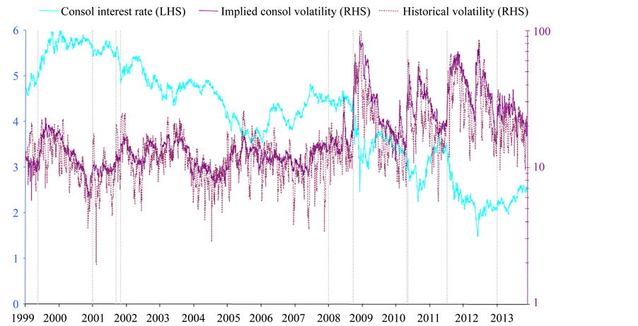
Figure 1. Consol rate and consol volatilities.
Second, our findings allow an homogeneisation of volatility measure (with a forward-looking feature), pro- viding information for the entire market without being restricted to one particular maturity or to the frequency of coupons/cash flows idiosyncratic to a particular benchmark instrument.
The restrictive nature of standard volatility measures (due to the strong link to a certain maturity and/or fre- quency) usually limit the use of volatility measure in times series regressions. The consol volatility provides new research avenues as regards volatility transmission and/or assessment of market stress.
Acknowledgements
The authors would like to thank colleagues of the ECB and the participants at the 7th Methods in International Finance Network (MIFN) Conference on 23-24 September 2013 for fruitful discussion and suggestions. A special thank to the anonymous referees of the ECB Working Paper Series and of the journal which allow to improve the paper with their helpful remarks.
References
- Brousseau, V. and Durré, A. (2013) Interest Rate Volatility: A consol Rate-Based Measure. ECB Working Paper Series 1505.
- Fisher, L. and Weil, R.L. (1971) Coping with the Risk of Interest-Rate. Journal of Business, 44, 408-431. http://dx.doi.org/10.1086/295402
- Heath, D., Jarrow, R. and Morton, A. (1992) Bond Pricing and the Term Structure of Interest Rates: A New Metho- dology for Contingent Claims Valuation. Econometrica, 60, 77-105. http://dx.doi.org/10.2307/2951677
- Duffie, D. and Kan, R. (1996) A Yield factor Model of Interest Rates. Mathematical Finance, 6, 379-406. http://dx.doi.org/10.1111/j.1467-9965.1996.tb00123.x
- Vasicek, O. (1977) An Equilibrium Characterization of the Term Structure. Journal of Financial Economics, 5, 177- 188. http://dx.doi.org/10.1016/0304-405X(77)90016-2
- Cox, J., Ingersoll, J. and Ross, S. (1979) Duration and the Measurement of Basis Risk. Journal of Business, 52, 51-61. http://dx.doi.org/10.1086/296033
- Brousseau, V. (2002) The Functional Form of Yield Curves. ECB Working Paper Series 148.
- Gourieroux, C. and Sufana, R. (2006) A Classification of Two-Fact or Affine Diffusion Term Structure Models. Jour- nal of Financial Econometrics, 4, 31-52. http://dx.doi.org/10.1093/jjfinec/nbj003
- Brousseau, V. and Durré, A. (2014) Sur une représentation paramétrique affine de la courbe des taux. Revue Bancaire et Financière, 4, 297-310.
Annex
Determination of the Consol Volatility
1. Data
1.1. Working Days and Instruments
The dataset contains all the TARGET working days from 4 January 1999 to 21 November 2013, so 3816 TAR- GET working days. The financial instruments belong to the OTC marke: short-term unsecured deposit of maturity 1-day, EONIA swaps from 1-week to 30-year, 6-month EURIBOR swaps for the corresponding ma- turities, at-the-money implied volatilities of EURIBOR swaptions with maturity 1-month to 5-year, and with underlying EURIBOR swap maturity 1-year to 30-year. Besides, the EONIA fixing is included in the dataset.
1.2. Raw Data
As the financial instruments taken into account are handled on the OTC market, we made use of quoted data, from which we retained only the mid. We gave a preference to quotes issued by the broker ICAP, and when not available, our primary fall-back was the generic quote of Reuters.
1.3. Completion
The data have been completed by reconstructed numbers in three cases.
・ When the history of long-term EONIA swaps was missing.
・ When the history of the options was missing.
・ When the history of an instrument was missing due to a London closing day, a case which occurred only in the recent years.
1.4. Descriptive Statistics of the Sample
The resulting data sample is described by the following descriptive statistics:
2. Algorithms
2.1. Yield Curves
2.1.1. Composition
The EONIA curve is made of short-term unsecured deposits of maturity 1-day (overnight, tom-next and spot- next) and of EONIA swaps from 1-week to 30-year.
The EURIBOR swap curve is made of short-term unsecured deposits of maturity 1-day (overnight, tom-next and spot-next) and longer (between 1-week and 6-month) and of swaps versus 6-month EURIBOR from 1-year to 30-year.
2.1.2. Bootstrapping
We turn now to the construction of the yield curve from a collection of interest rate instruments. The con- struction of the yield curve consists into the successive calculation of zero-coupon prices or “discount factors”, is termed “bootstrapping”. For a detailed description of the bootstrapping, we refer to [7] 9, [9] . The algorithm should be such that:
・ it re-prices all the instruments contained in the above described yield curves to their exact original observed price;
・ it can be entirely described through a finite (albeit not a priori specified) number of rates and dates.
The instruments are sorted by ascending maturity. One constructs the curve by recurrence up to each maturity. Each of those maturities is termed a “knot point”. Rates at intermediate points on the curve can be estimated by assuming a shape for the curve either in zero-coupon price or rate space. The choice of that interpolation rule constitutes the signature of the bootstrapping method. This choice is not conditioned by any theoretical reason, but by several practical reasons. The chosen rule should be such that:
1) The curve is smooth.
2)The curve does not have strong oscillations.
To those requirements, we add the supplementary one that:
3) The integral of the zero-coupon price between two knots can be computed in closed analytical form. The same holds for the integral of the zero-coupon price multiplied by the time to maturity.
The two first conditions are antagonist: an interpolation rule that favours one requirement will generally disfavour the other one.
The third requirement reflects the necessity of performing consol-related calculations, to be described in paragraph 2.3.2..
We have tested four different rules, satisfying to those three criteria, among which the “unsmoothed Fama- Bliss” bootstrapping, whose interpolation rule results into stepwise constant forward rates. All of the methods performed close in term of the realistic aspect of the constructed curve. On the basis of some minute differences, we have chosen as default bootstrapping method one of the three other methods, namely, the one used in [9] .
2.1.3. Extrapolation
It order to handle swaptions of maturity 5-year on 30-year swaps, one needs a yield curve covering a range of 35 years. Yet, quotes for the EONIA swaps stop at the 30-year tenor, at least for the price source that we have chosen to privilege. We have therefore extrapolated the EONIA curve.We have chosen to also extrapolate the EURIBOR swap curve to 35-year, to ensure the similarity of their treatment. The extrapolation of a curve has been achieved by adding the zero-coupon rate z(35) defined as 2 × z(30) − z(25).
2.2. Implied Volatilities
2.2.1. Converted Volatilities
The primary input for the calculation of the consol volatility is a set of implied volatilities quoted in the market. The implied volatilities that we have used as raw data are those of EURIBOR swaptions, which are standardized options on 6 month EURIBOR swaps. They cannot be directly used, and this, for two reasons.
Firstly, the swaptions volatilities are implied by a Black and Scholes model in which the logarithm of the swap rate is assumed to be a Brownian motion. By contrast, while the consol volatility, resulting from the equ- ations presented in the text, has to be implied by a Black and Scholes model. A conversion will thus be necessary, changing the raw swaptions volatilities into other ones implied by the second model.
Secondly, the swaptions volatilities pertain to EURIBOR-linked instruments, whereby the consol volatility pertains to the EONIA curve.
The change of model cannot be done by an exact calculation (or that exact calculation would be too com- plicated). However, as we already mentioned, we know that the motion of the empirical yield curves are pri- marily composed of parallel shifts. We then make an approximation and assume that those movements consist purely of parallel shifts. Thus, we only need to do the calculation at the first order, i.e. to multiply the raw swap- tions volatility by the sensitivity of the log zero coupon price w.r.t. the log swap rate.
The two conversions are simultaneously achieved as follows:
The underlying of the option―which is a forward EURIBOR swap―is priced from the EURIBOR curve. Then, one computes the quantity of parallel shift to apply to the EONIA curve to let it price the forward swap at its present market price. That quantity is called the “z-spread”, we denote it with h.
The sensitivity of the log zero coupon price (of the EONIA curve) w.r.t. the log swap rate (non compounded, with day-count actual/360) is then given by:
 (1)
(1)
where:
・
 refers
to the time-to-maturity of the option.
refers
to the time-to-maturity of the option.
・
 is
the time-to-maturity of the swap (for instance 35-year for a 30-year swap forward
in 5-year).
is
the time-to-maturity of the swap (for instance 35-year for a 30-year swap forward
in 5-year).
・
 is
the swap rate (non compounded, with day-count actual/360),
is
the swap rate (non compounded, with day-count actual/360),
 is
the swap's z-spread to EONIA curve (continuously compounded, with day-count actual/365),
and
is
the swap's z-spread to EONIA curve (continuously compounded, with day-count actual/365),
and
・
 is
the swap rate (non compounded, with day-count actual/360) of a forward swap having
z-spread
is
the swap rate (non compounded, with day-count actual/360) of a forward swap having
z-spread
 w.r.t. the EONIA curve (so that
 ).
).
The product of the quoted volatility by this sensitivity yields a first order approximation of the “converted volatility”. To be on the safe side, we actually used a higher order approximation (up to the 5-th power of the quoted volatility). However, that higher precision does not bring any visible difference.
We denote the “converted volatility” with .
For an instantaneous volatility
.
For an instantaneous volatility ,
we will use the short-hand
,
we will use the short-hand .
.
2.2.2. Instantaneous Volatilities
We are then left with a collection of implied volatilities for options tenors ranging between 1-month and 5-year.
We need to obtain instantaneous volatilities, i.e. the limit of the at the money volatility tends to zero. Instan- taneity as meaning, in concrete terms, the interval between two subsequent TARGET working days. This im- plies that we reconstruct at the money volatilities of tenor one TARGET working day.
This is achieved by creating the cubic spline of the converted volatilities of tenors ranging between 1-month and 5-year and by extrapolating the resulting splined function to the tenor 1-day. The quantity to be splined is not directly the converted volatility, but the squared converted volatility multiplied by the time to maturity.
2.3. Consol-Related Calculations
2.3.1. Formulas
The consol rate, consol duration, consol ksi and consol volatility rely on the computation of three integrals:
 (2)
(2)
 (3)
(3)
 (4)
(4)
where
 is the zero coupon price for time-to-maturity
 ,
and
,
and
 is the zero coupon price instantane- ous volatility for time-to-maturity
 . The notation
 ,
without argument, designates the consol volatility.
,
without argument, designates the consol volatility.
The computation of the consol rate, denoted with ,
the consol duration, denoted with
,
the consol duration, denoted with ,
and the consol ksi, denoted with
,
and the consol ksi, denoted with ,
boils down to the formulas:
,
boils down to the formulas:
 (5)
(5)
 (6)
(6)
 (7)
(7)
Consistently with what we did for the conversion of volatilities, we will assume
that the yield curves move- ments consist purely of parallel shifts. With the help
of that approximation, that we use for the second time, the
 under the integral sign in (4) can be interpreted as scalars instead of vectors.
The consol volatility is given by the formula:
under the integral sign in (4) can be interpreted as scalars instead of vectors.
The consol volatility is given by the formula:
 (8)
(8)
The ,
even when we made them scalar numbers, have to be determined on the basis of the
instan- taneous volatilities resulting from the procedure described in 6. Yet those
ones exist for eleven tenors of the underlying swaps, ranging from 1-year to 30-year.
We take recourse again to a spline procedure, whereby we add to the list of available
tenors the artificial tenor zero-day. For now, the quantity to be splined is directly
the instantaneous volatility, and not the squared one multiplied by the time to
maturity.
,
even when we made them scalar numbers, have to be determined on the basis of the
instan- taneous volatilities resulting from the procedure described in 6. Yet those
ones exist for eleven tenors of the underlying swaps, ranging from 1-year to 30-year.
We take recourse again to a spline procedure, whereby we add to the list of available
tenors the artificial tenor zero-day. For now, the quantity to be splined is directly
the instantaneous volatility, and not the squared one multiplied by the time to
maturity.
To compute the consol volatility of the theoretical yield curves of the affine models, used in the simulations, we start from the identity:
 (9)
(9)
where V designates the volatility of the vector of factors: V is either
 for the 1-factor case or
 for
the 2-factor case. The operator
for
the 2-factor case. The operator
 represents the gradient w.r.t. the vector of factors.
For the 1-factor model, the
 is anyway a scalar, and for the 2-factor model, the
 is a vector of dimension 2, but both components can be explicitly computed.
2.3.2. Numerical Implementation
For what regards the consol rate, duration and ksi, in the case of the curves bootstrapped from empirical data, we have analytically computed the integrals between subsequent knot points of the bootstrapping. To complement the integral between 35-year and infinity, we have assumed that the zero-coupon rate remained constant.
For what regards the consol rate, duration and ksi, in the case of the affine model curves, and for what regards the consol volatility, in both cases of empirical curve and model curve, we have discretized the integrals with a step of 30 calendar days and we have computed 1000 steps, reaching a maturity of circa 80-year. To comple- ment the integral between that latest maturity and infinity, we have assumed that the zero-coupon rate remained constant, and that the instantaneous volatility remained strictly proportional to the time-to-maturity.
2.3.3. Consol Performance and Numerical Performance
Let
 and
and
 to consecutive TARGET working days. The excess return between
 and
and
 then writes:
 (10)
(10)
where CONSOL(t), is the consol rate observed at the close of business of t, continuously
compounded, with a day count actual/365, and expressed in percentage points. The
normalized excess return is the quotient of the excess return between
 and
and
 and of the consol volatility observed at the close of business of
 .
.
NOTES

*Corresponding author.

1See also the discussion on the relevance and the scope of the various volatility measures in [1] .
2For example, a bond observed at time t and having maturity date T shall
have a time to maturity
 satisfying to the relation:
 .
.

3Such a normalisation is needed given the perpetual nature of this bond.
4By construction, the consol rate corresponding to a flat consol yield curve is equal to the level of that yield curve.

5Affine models represent the yield curve as determined by a finite number of state variables, called factors, in such a way that the curve is an affine function of those factors.
6By definition, two probabilities are said to be equivalent if and only if they are defined on the same σ-algebra and, furthermore, they attribute the weight zero or the weight one to the same measurable sets.
7The solution of a SDE consists of a measure on the set of future trajectories―endowed with some suitable σ-algebra―and is therefore the relevant concept when defining expectations, which are essentially integrations w.r.t. that measure.

8When v is not equal to zero. The DK1 model can be rewritten as a parallel shift of the CIR model.

9See paragraph 3.2.2., pp. 19-20.