ABSTRACT

Wavelet methods are a very useful tool in solving integral equations. Both scaling functions and wavelet functions are the key elements of wavelet methods. In this article, we use scaling function interpolation method to solve Volterra integral equations of the first kind, and Fredholm-Volterra integral equations. Moreover, we prove convergence theorem for the numerical solution of Volterra integral equations and Freholm-Volterra integral equations. We also present three examples of solving Volterra integral equation and one example of solving Fredholm-Volterra integral equation. Comparisons of the results with other methods are included in the examples.

1. Introduction

The study of finite-dimensional linear systems is well developed. As an infinite-dimensional counter part of finite-dimensional linear systems, one can view integral equations as extensions of linear systems of algebraic equations. An integral equation maybe interpreted as an analogue of a matrix equation which is easier to solve. There are many different ways to transform integral equations to linear systems. Many different methods have been used for solving Volterra integral equations and Freholm-Velterra integral equations numerically.

In this paper, we first recall the method of scaling function interpolation. Then we solve linear Volterra integral equation of the form:

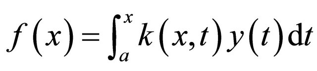(1)

and Fredholm-Volterra integral equations of the form:

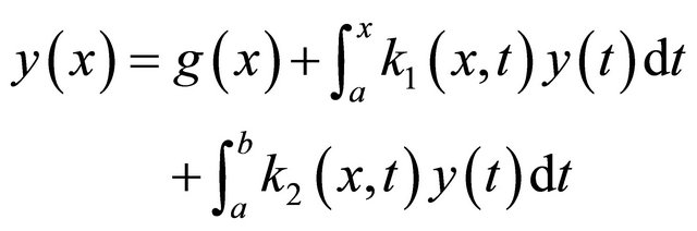(2)

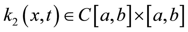
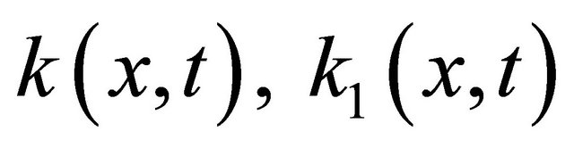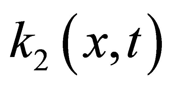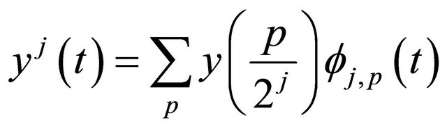
where the functions and are known functions and called kernels. The function is known, and the function is to be determined. One of the motivations in this study arose from equations in theoretical physics. In fact, there are many applications in several disciplines as well. We will use scaling function interpolation method to solve integral equations. As a natural question, one would wonder any possible convergence properties and how this method would compare with other methods. We will prove two convergence theorems and present several examples.

2. Approximation

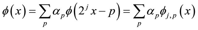
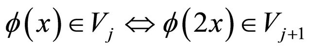
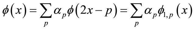
Wavelets and scaling functions are a useful tool in approximation methods of solutions of differential and integral equations [1]. We first recall Multiresolution analysis (MRA) [2]. We assume the scaling function and wavelet function f, Ψ are sufficiently smooth and satisfy MRA with compact support and Ψ has N vanishing moments (defined below). The scaling function is defined as

(3)

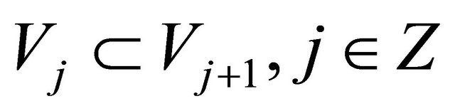
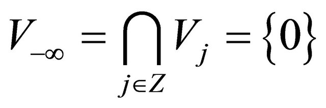
for some coefficients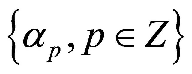. By using this dilation and translation we defined a nested of sequence spaces 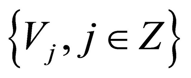which is called MRA of with the following properties:

(4)

(5)

is dense in  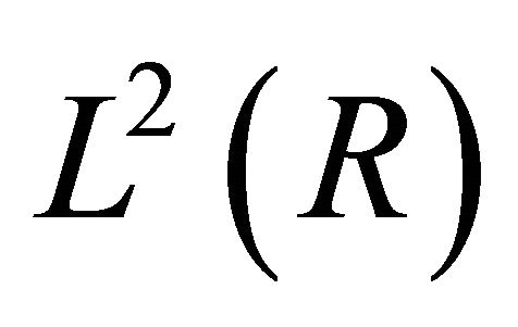        (6)

. (7)

For the subspace is built by,

then 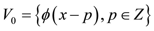and 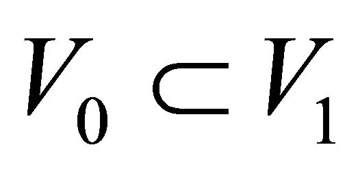we can write

. In general,

. (8)

In fact, for each j we define the orthogonal subspace of in the subspace, the or thogonal basis of is denoted by

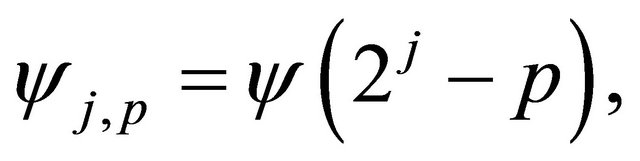(9)

and the wavelet function can be obtained by

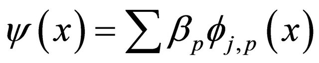. (10)

for some coefficients. Some interesting properties of scaling and wavelet functions make wavelet method more efficiently than other methods such as spline approximations in solving an equation. A lot of computational time and storage capacity can be saved since we do not require a huge number of arithmetic operations partly due to the following properties.

Vanishing moments:

(11)

and in this case the wavelet is said to have a vanishing moment of order k.

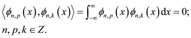
Semiorthogonality:

(12)

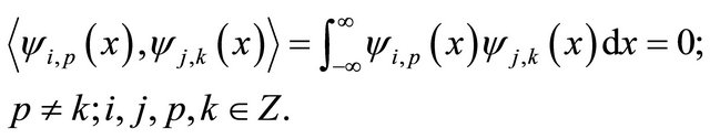
The set of scaling functions is orthogonal at the same level n, which means:

(13)

Coiflet (of order L) has more symmetries and it is an orthogonal multiresolution wavelet system with,

. (14)

. (15)

where is the moment of scaling functions.

3. Scaling Function Interpolation

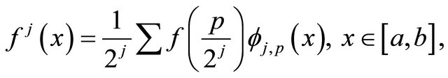
In MRA, any given function can be interpolated by using the basis functions in the subspace as follows:

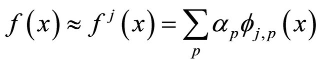(16)

where the coefficientsv are evaluated by using the semiorthogonality of the scaling functions (12) such that

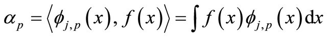. (17)

Hence the Equation (16) becomes as follows:

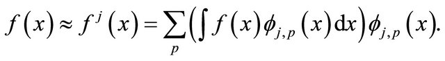
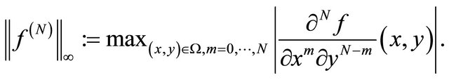
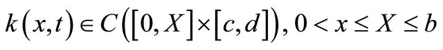
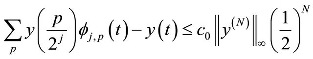
To approximate a given function f, one can use sampling values of f at certain points. It is proved in [3], namely, an interpolation theorem using coiflet, namely, if and are sufficiently smooth and satisfy the Equations (10)-(15) and the function, where Ω is a bounded open set in R², , then,

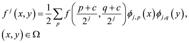(18)

where the index set is

.

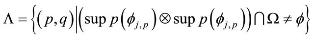In addition, the moment satisfies

.

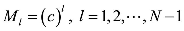Then 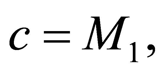and

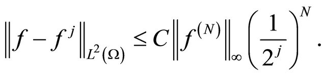
where C is a constant depending only on N, diameter of Ω and

For one-dimensional analogue, we have

(19)

and

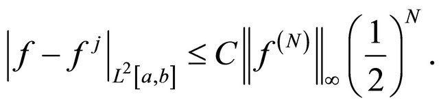(20)

where

4. Solutions of Linear Integral Equation

In this section, Coiflet is used to solve linear integral Equations (1) and (2), where we will explain the method in terms of matrix notation.

4.1. Linear Volterra Integral Equation

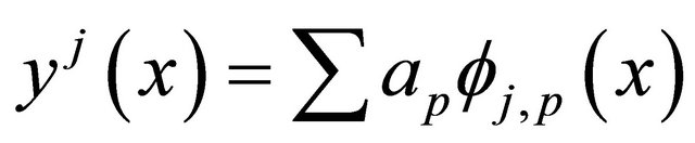
In this subsection we will use the interpolation Formula (19) to solve Volterra integral Equation (1). The unknown function in Equation (1) can be expressed in term of scaling functions in the subspace such that

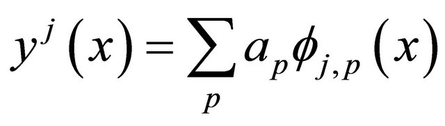. (21)

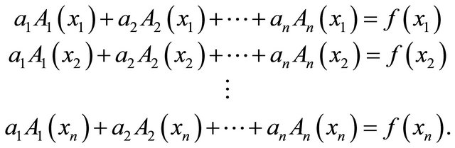
By substituting Equation (21) into the Equation (1), we have the following system,

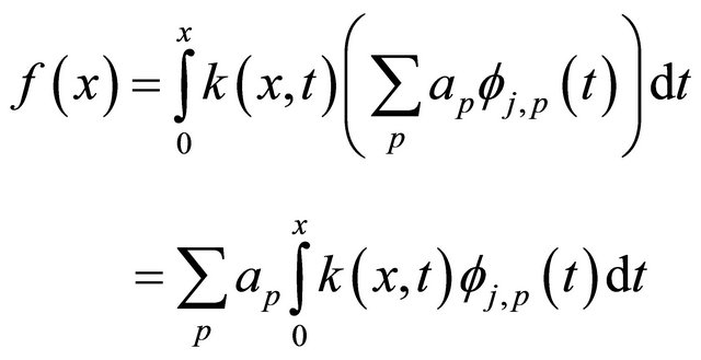(22)

To simplify the system, let

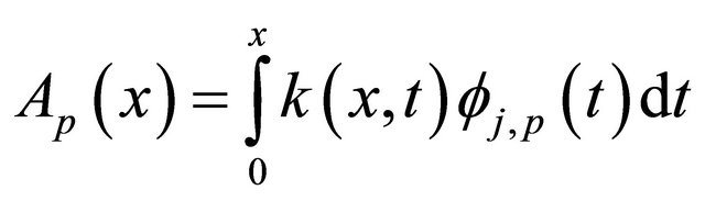
Then the system (22) becomes

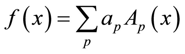. (23)

The coefficients 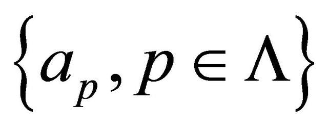can be evaluated by substituting the set of real numbers

into the system (23), let, then the system (23) can be written in the form

If we use the notation 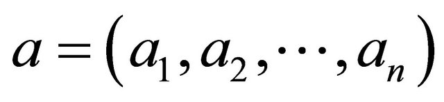and

, then the system (23) is equivalent to the system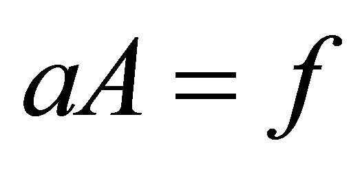, and the solution is

. (24)

This gives raise to coefficients in (23) and we obtained a numerical solution to Equation (1).

4.2. Linear Fredholm-Volterra Integral Equation

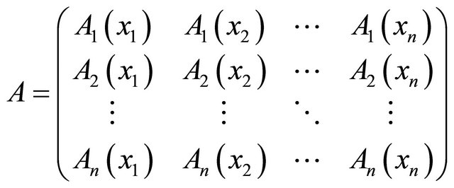
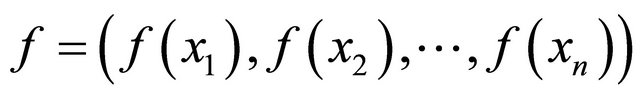
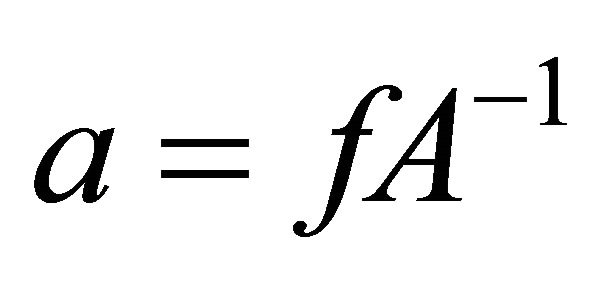
To solve the Fredholm-Volterra integral Equation (2), we use a similar algorithm as we use in 4.1. The unknown function can be approximated by using Equation (1) and one can have the system of linear equations;

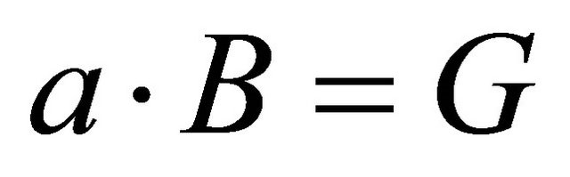
where a is the vector of unknowns as we introduce in Equation (21),

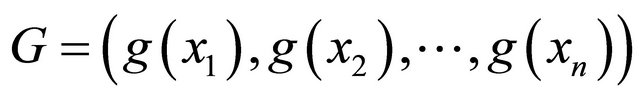
and

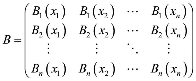
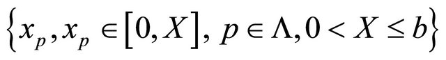
with

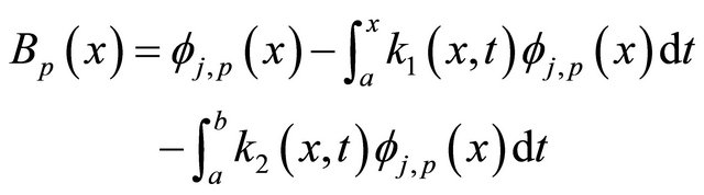
and the set of 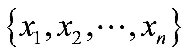is in the interval which one can be choose equally spaced. In the next section we will discuss the convergence for the method by deriving a convergence theorem of this numerical solution.

5. Error Analysis

In this section, we provide with the convergence rate of our method for the numerical solution of solving linear Volterra integral equations and Freholm-Volterra integral equation respectively. We will explain the necessary conditions for the convergence.

Theorem 5.1

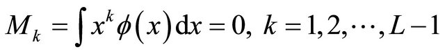
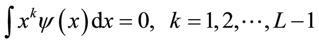
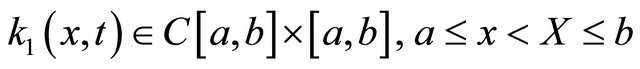
In Equation (1), suppose that the functions

,

and the two functions, are in, for

.

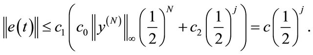
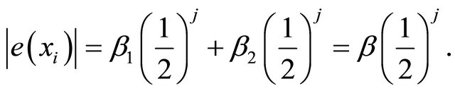
If an approximate solution of the Equation (1) with coefficients obtained in (24), and the error at the point

is. Then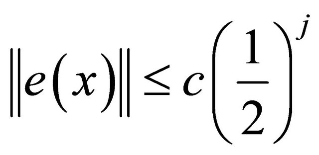where c is a constant.

wang#title3_4:spProof:

We begin with the following equation.

. (25)

At any point 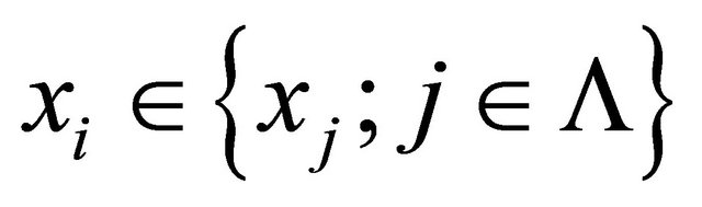Equation (25) becomes:

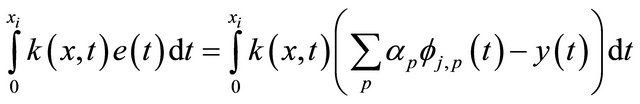then

. (26)

For

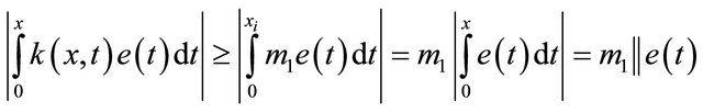
Then,

(27)

Such that.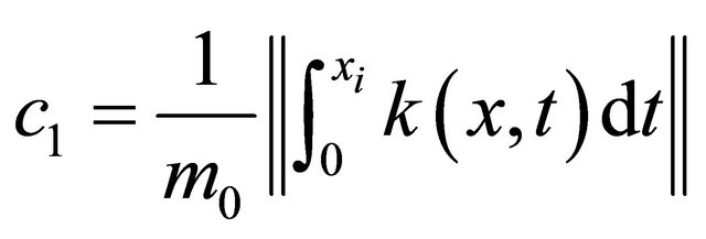

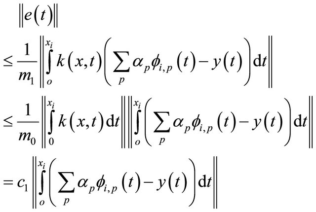
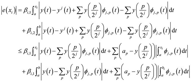
By (19), the unknown function can be interpolated by using the coiflet such that:

(28)

If we add and subtract Equation (28) in Equation (27), we get the following inequality:

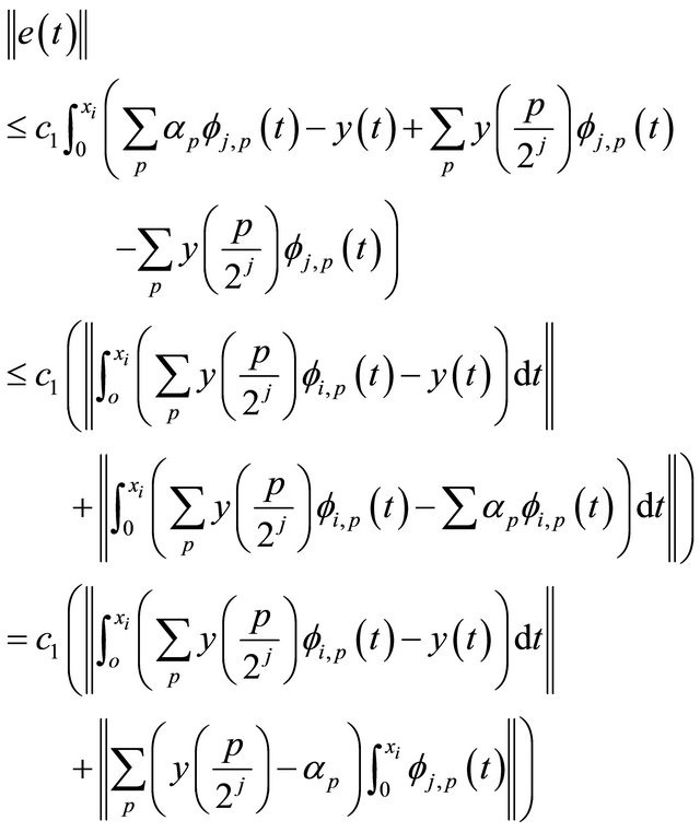
But by (20), we have that;

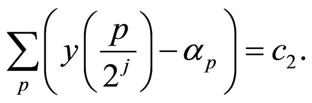
And since 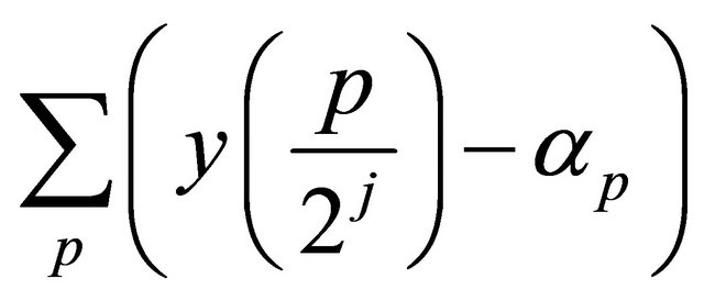is finite then denote it as

By using the above results and the orthonomality of the scaling functions, we conclude that

Theorem 5.2

In Equation (2), suppose that the functions

,

, and are in

, for

If an approximate solution of the Equation (2) with coefficients obtained in (24), and the error at the point is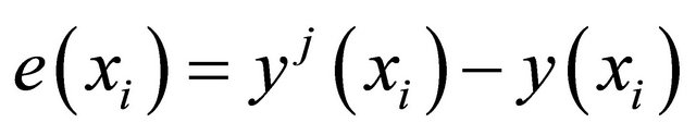. Then

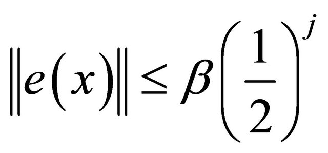, where β is a constant

wang#title3_4:spProof:

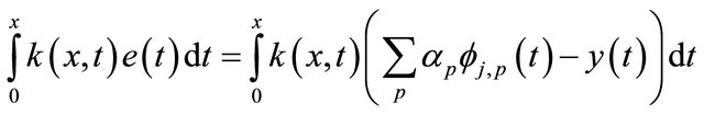
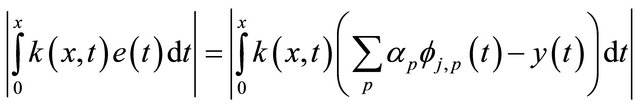
Substitute (21) into Equation (2), we get the following integral equation

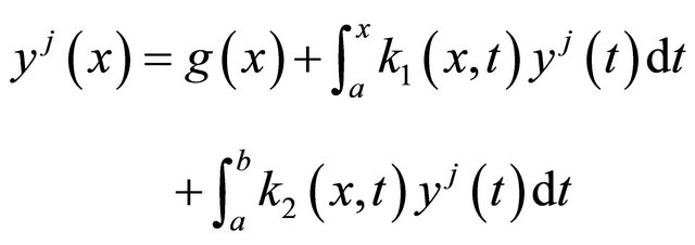(29)

Subtracts Equation (27) from (1) and substitute x by x_i to get;

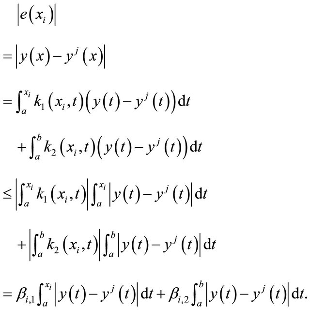(30)

Add and subtract Equation (28) for absolute value in the previous equation, we get the following equation.

(31)

We use the same idea in the proof of 5.1, and obtain the following error estimate.

Remark

Here we discuss only the case when the kernel function is positive. We can generalize our method for any given continuous function in Equation (1);

1) If is positive, we have obtained the convergence theorem.

2) If is negative then let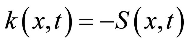, then the function is positive and we can apply our method for the equation 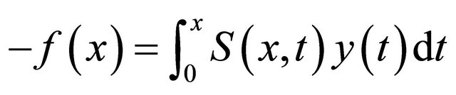which has the same solution as the Equation (1).

3) If the function is neither of the above two cases, the function can be written as a sum of two positive functions where

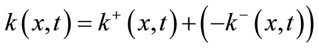
Then Equation (1) becomes

And hence the result is concluded in a similar fashion.

6. Numerical Examples

In the following examples, we will solve several linear Volterra integral equations of the first kind and Fredholme-Volterra integral equations using coiflet of order 5 and provide the absolute errors. The examples (1-3) are also shown in [4] and the example 4 is presented in [5]. We will compare our results with others and show that our method has better approximations than other methods.

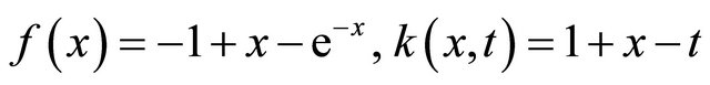
Example 1

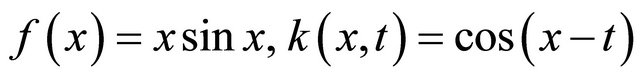
Consider the integral Equation (1) with;

and the exact solution is

. The numerical results are presented in Table 1.

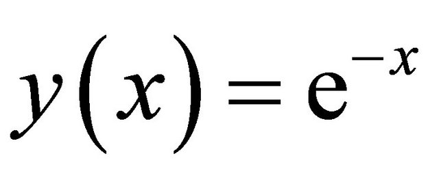
Example 2

Consider the integral Equation (1) with;

and b = 1, and the exact solution is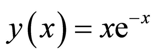. The numerical results are presented in Table 2.

Example 3

Consider the integral Equation (1) with;

and the exact solution is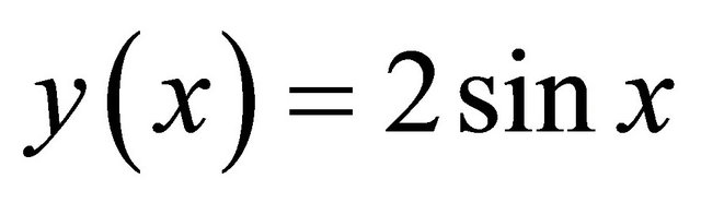. The numerical result are presented in Table 3.

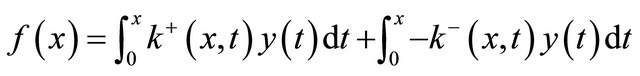
Example 4

Consider the integral Equation (2) with;

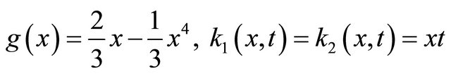and the exact solution is 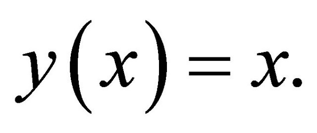The numerical results are presented in Table 4.

Table 1. The absolute errors for example 1.

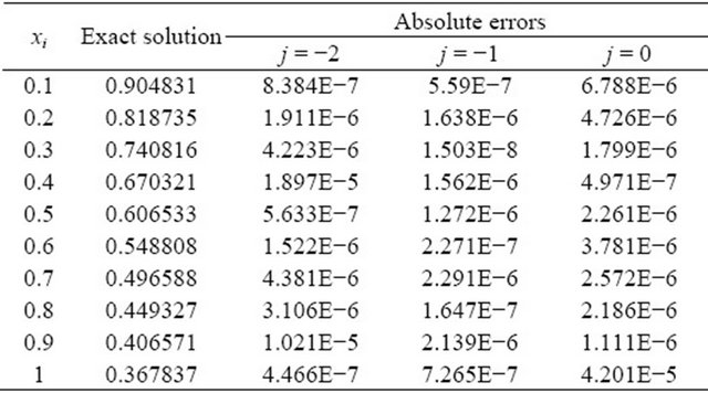
Table 2. The absolute errors for example 2.

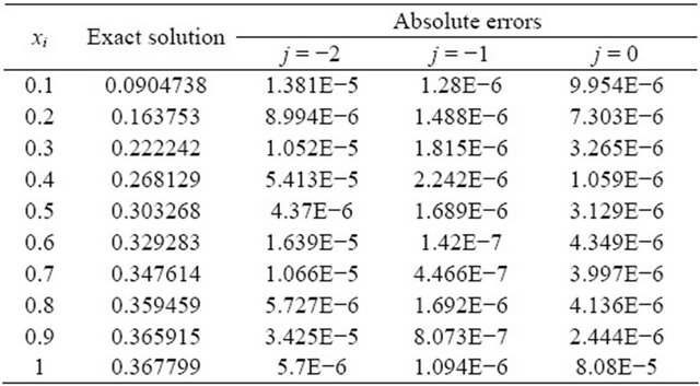
Table 3. The absolute errors for example 3.

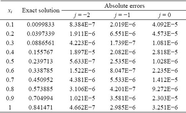
Table 4. The absolute errors for example 4.

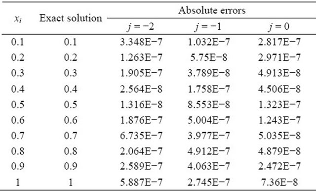
In the above tables, we use the notation E − n which denotes and j denotes the level of MRA.

7. Concluding Remark

In this paper we have shown a better method in solving Volterra integral equations of the first kind, and Fredholm-Volterra integral equations. We also prove convergence theorem for the numerical solution of Volterra integral equations and Freholm-Volterra integral equations respectively. It would be interesting to extend the results to two-dimensional case for the above mentioned equations and apply to some imaging problems.

REFERENCES

- E. B. Lin and N. Liu, “Legendre Wavelet Method for Numerical Solutions of Partial Differential Equations,” Numerical Methods of Partial Differential Equation, Vol. 26, No. 1, 2010, pp. 81-94. doi:10.1002/num.20417
- C. K. Chui, “In Introduction to Wavelets,” Academic Press, Boston, 1992.
- E. B. Lin and X. Zhou, “Coiflet Interpolation and Approximate Solutions of Elliptic Partial Differential Equations,” Methods for Partial Differential Equations, Vol. 13, No. 4, 1997, pp. 302-320.
- M. T. Rashad, “Numerical Solution of the Integral Equations of the First Kind,” Applied Mathematics and Computation, Vol. 145, No. 2-3, 2003, pp. 413-420. doi:10.1016/S0096-3003(02)00497-6
- A. S. Shamloo, S. Shaker and A. Madadi, “Numerical Solution of Fredholm-Volterra Integral Equation by the Sunc Function,” American Journal Computation Mathematics, Vol. 2, No. 2, 2012, pp. 136-142. doi:10.4236/ajcm.2012.22019