International Journal of Geosciences
Vol.4 No.1A(2013), Article ID:27426,8 pages DOI:10.4236/ijg.2013.41A023
Characterizing Potential Fishing Zone of Skipjack Tuna during the Southeast Monsoon in the Bone Bay-Flores Sea Using Remotely Sensed Oceanographic Data
Faculty of Marine Science and Fisheries, Hasanuddin University, Makassar, Indonesia
Email: mukti_fishocean@yahoo.co.id, mukti@unhas.ac.id
Received November 28, 2012; revised December 28, 2012; accepted January 18, 2013
Keywords: Skipjack Tuna; Satellite Data; Generalized Additive Model; Linear Model; Upwelling; Potential Fishing Zones; Bone Bay and Flores Sea; Southeast Monsoon
ABSTRACT
Potential fishing zones for skipjack tuna in the Bone Bay-Flores Sea were investigated from satellite-based oceanography and catch data, using a linear model (generalized linear model) constructed from generalized additive models and geographic information systems. Monthly mean remotely sensed sea surface temperature and surface chlorophyll-a concentration during the southeast monsoon (April-August) were used for the year 2012. The best generalized additive model was selected to assess the effect of marine environment variables (sea surface temperature and chlorophyll-a concentration) on skipjack tuna abundance (catch per unit effort). Then, the appropriate linear model was constructed from the functional relationship of the generalized additive model for generating a robust predictive model. Model selection process for the generalized additive model was based on significance of model terms, decrease in residual deviance, and increase in cumulative variance explained, whereas the model selection for the linear model was based on decrease in residual deviance, reduction in Akaike’s Information Criterion, increasing cumulative variance explained and significance of model terms. The best model was selected to predict skipjack tuna abundance and their spatial distribution patterns over entire study area. A simple linear model was used to verify the predicted values. Results indicated that the distribution pattern of potential fishing zones for skipjack during the southeast monsoon were well characterized by sea surface temperatures ranging from 28.5˚C to 30.5˚C and chlorophyll-a ranging from 0.10 to 0.20 mg·m−3. Predicted highest catch per unit efforts were significantly consistent with the fishing data (P < 0.01, R2 = 0.8), suggesting that the oceanographic indicators may correspond well with the potential feeding ground for skipjack tuna. This good feeding opportunity for skipjack was driven the dynamics of upwelling operating within study area which are capable of creating a highly potential fishing zone during the southeast monsoon.
1. Introduction
The Bone Bay-Flores Sea located in the central Indonesian Seas is one of the most biologically productive areas in the tropical region (Figure 1). This area is also one of the main pathways the Indonesian throughflow (ITF) and is strongly influenced by the Asian monsoon i.e. southeast monsoon and northwest monsoon [1]. The interacttion of the ITF and the Asian monsoon affect the specific current circulation system, Ekman mass and heat transport, tidal mixing, wind induced upwelling and downwelling system and environmental variability of sea surface temperature (SST), salinity and surface chlorophylla concentration [1-3]. The dynamics of the physical oceanographic structures in this area, results in a highly productive habitat, which serves as a feeding ground for various commercially and ecologically important species such as skipjack tuna, yellowfin tuna and flying fish [4- 6].
The biophysical environment characteristics of the Bone Bay-Flores Sea play an important role in serving this area as one of the most productive skipjack tuna fishing grounds in Indonesia Seas. Several oceanographic studies found that the migration, distribution and abundance of skipjack are highly associated with oceanic fronts and eddy [7,8]. The distribution of the 29˚C SST isotherm is a reasonable proxy to detect the region of highest skipjack CPUEs (frontal area) in western Pacific Ocean [9]. The highest skipjack CPUEs off the southern Brazilian coast are obtained in waters of SST 22˚C - 26.5˚C, although that relationship varies seasonally [10].
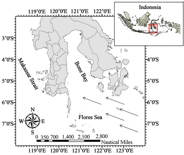
Figure 1. Location map of the area investigated within Indonesian Waters. Black arrows indicate the upstream direction of the wind-induced upwelling during the southeast monsoon.
The recent studies concluded that SST and surface chlorophyll-a are the most two important habitat predicttors for skipjack tuna migration in the western North Pacific Ocean [11]. SST plays an important role in tuna physiology, and temperature variations are often linked with the biological richness of an oceanic area [12]. Surface Chl-a is known as a very important oceanographic parameter in determining the primary production level. In the oceanic environment, surface chlorophyll-a is often considered as an index of biological productivity and it could be related to fish production [13]. A Combination of the SST and Chl-a can complement one another for determining potential fishing ground for tuna [14]. Most investigations suggest that SST and chlorophyll-a play a key in stimulating distribution patterns and variability of tuna abundance in sub-tropical waters. However, the motivating questions remain are how the distribution pattern of potential fishing zones for skipjack tuna in the tropical region particularly in Indonesian Seas and what is the important oceanographic factor controlling the skipjack tuna abundance. Therefore, the objectives of this work were to study skipjack tuna potential fishing zone and to characterize the oceanographic factors controlling the potential fishing zone from satellite-based oceanography and fishery data, using statistical models and geographic information systems (GIS).
2. Data and Methods
2.1. Fishery Data
The scientific survey has been conducted in the Bone Bay-Flores Sea during the southeast monsoon (AprilAugust) to collect the fishery and oceanographic data. The study data were obtained by following pole and line fishing operations together with fishermen during the period. We recorded all the data for each fishing operation. The data comprised daily geo-referenced fishing positions (latitude and longitude), catch in number of skipjack and effort (fishing set), from which catch per unit effort (CPUE) was determined in number of fish per setting (fishing operation). The data were mapped using ARCGIS 9.2 (ESRI, Redlands, CA, USA) and further compiled into monthly resolution datasets. The field oceanographic data were used to validate the accuracy of satellite data.
2.2. Remotely Sensed Environmental Data
Remotely sensed physical and biological environmental data used to describe the oceanographic conditions at and around the skipjack tuna fishing grounds were sea surface temperature (SST) and Chl-a concentration. All SST and Chl-a data were estimated from Aqua/MODIS with monthly mean temporal resolution and 0.04 degree (4 km) of longitude and latitude spatial resolution. The satellitederived environmental data distributed by the Goddard Space Flight Center of the National Aeronautics and Space Administration (NASA) with Standad Mapped Image (SMI) level 3 binary data using HDF file. This study processed the satellite remotely sensed environmental data that have same period with the fishery data, from April to August 2012. Data were matched to corresponding images for both SST and surface Chl-a using the Interactive Data Language (IDL) program/script. The program was made in latitude and longitude positions from the fishery dataset. The datasets were then used to develop the statistical predictive models. All environmental data and predicted CPUE derived GAM-linear model were mapped using ArcGIS 9.2.
2.3. Construction of GAM and GLM
To predict spatial patterns of potential fishing zone for skipjack tuna, statistical models were applied. These models were built by combining generalized additive model (GAM) and linear model/generalized linear model (GLM). This study constructed the linear model based on the nature of the relationship between skipjack CPUE as the response variable and SST and Chl-a as predictor variables resulting from a GAM with the least different of residual deviance [15,16]. Despite the GAM may explain variance of CPUE more effective and flexible than the linear model (GLM), the model has no analytical form [16]. A linear model provides a way of estimating a function of mean response (CPUE) as a linear function of some set of covariates. Therefore, this study used the GLM fit to predict a spatial pattern of skipjack CPUE.
The first step to get the spatial predictive model was to construct GAM as an exploratory tool. This step was used to identify the shapes of the relationships between environmental factors and skipjack CPUE as it was most likely that the expected relationships are non-linear. The second, once the shape of the relationships between the skipjack CPUE and each predictor (SST and Chl-a) were identified, the appropriate functions were used to parameterize these shapes in the linear model [5]. The shapes resulting from the GAM were reproduced as closely as possible using the piecewise linear model. Statistical Models of the GAM and the linear model respectively shown in Equations (1) and (2) were applied:
 (1)
(1)
 (2)
(2)
where α and β0 are constant, s(.) is a spline smooth function of the predictor variables (SST and Chl-a) and ε is a random error term, β1 and β2 is the vector of model coefficients. The constant intercept terms were computed using gam and glm functions in S-PLUS. All statistical analyses were carried out in S-PLUS 2000.
Skipjack CPUE follows a continuous distribution, this work fit the GLM using a normal distribution as the family associated with identity link function [17]. The data distribution and the link function in the linear model/ GLM were exactly same as those used in the GAM. A logarithmic transformation of the CPUE was used to normalize asymmetrical frequency distribution, and this study added a value of one to all CPUE values to account for zero CPUE data. The model selection process for the best predictive model for explaining CPUE data was based on forward and backward stepwise manner. The predictors for final model were considered to be significant for explaining the variance of CPUE, if the residual deviance and Akaike Information Criteria (AIC) decrease, an increase in cumulative variance explained with each addition of the variables and the significance of final model term was lower than 0.01 (P < 0.01).
3. Results and Discussion
3.1. Spatial and Temporal Skipjack CPUE Distribution Pattern
Figures 2 and 3 show the monthly spatial distribution of pole and line fishery from April to August 2012 relative to oceanographic variables observed from satellite remote sensing. SST was highest during April-May and the relatively lower SST was more apparent during the season of high abundance (June-August) (Figures 2 and 4). During April-May, the fishing fleets occupied areas where SST ranged from 30.0˚C to 32˚C when the skipjack CPUEs were found in relatively lower than the three subsequent months.

Figure 2. The spatial distribution of skipjack CPUE (skipjack/fishing sets) from the pole and line fishery shown as dots for April-August, 2012 overlain on the MODIS SST images.

Figure 3. The spatial distribution of skipjack CPUE (skipjack/fishing sets) from the pole and line fishery shown as dots for April-August, 2012 overlain on the MODIS chlorophyll concentration images.
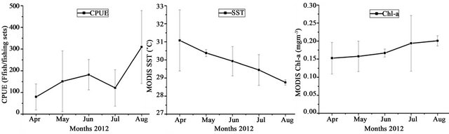
Figure 4. Monthly mean temporal variability of skipjack CPUE (left), SST (middle) and Chl-a (right) during the southeast monsoon (April-August).
Figure 2 shows that during the peak season (JuneAugust), the fishing operations aggregated in warm water of SST 28.5˚C to 30˚C when the highest CPUEs occurred. Fishing data CPUE are often used as an index of fish occurrence and abundance [18] and therefore high CPUEs can be said to indicate preferred oceanographic conditions for a species [15]. Whilst, fishing groundchlorophyll environment relationship during April-August showed that most fishing sets have a good association with surface chlorophyll-a of 0.11 mg·m−3 - 0.275 mg·m−3 (Figure 3). Specifically, during April-May, the highest frequency of fishing sets occurred in areas where Chl-a ranged from 0.10 mg·m−3 to 0.18 mg·m−3, and during the stronger effect of the southeast monsoon (June-August), it occupied mainly from 0.180 mg·m−3 to 0.275 mg·m−3. The latitudinal displacement of the fishing sets during the peak season corresponded with the spatial dynamics of relatively higher Chl-a concentration than during April-May. Figures 3 and 4 showed the highest CPUEs during the peak season were consistent with the increase of surface chlorophyll-a. These evidences reflects that the Chl-a and SST signatures are capable of detecting potential habitats (hotspots) such as upwelling area, frontal zone and eddy field for tuna species [11,19].
It was interesting to note that the period of June-August corresponded well with the increasing skipjack CPUE (Figure 4). The peak of southeast monsoon occurred from June to August as it was confirmed by the previous studies [1,3]. During that period, the skipjack tuna fishing grounds appeared to show the latitudinal displacement. In June and August, highly productive fishing grounds were mainly occurred in area of 121˚E - 121.5˚E and 4˚S - 4.5˚S. The fishery following the potential fishing zones displacement, moved to the north in response to the progression of relatively high Chl-a and decreasing gradually SST in July (Figures 2 and 3) and then back to reach the potential fishing grounds in the southeastern Bone Bay in August. Hence, this study suggested that spatial dynamics of skipjack tuna schools corresponded well with the specific area of the warm water SST and relatively high Chl-a concentration.
It is important to note that the highest skipjack CPUEs during the peak season are well characterized by the warm water SST of 28.5˚C - 30˚C and surface Chl-a of 0.15 mg·m−3 - 0.20 mg·m−3 (Figures 2-4). In general, the high CPUE in the Bone Bay-Flores was in accordance with the increasing surface Chl-a (>0.15 mg·m−3) and warm SST, reflecting that skipjack prefer the area of good physiological and trophic conditions. The decreasing trend of SST and the increase in chlorophyll concentration during June-August offer the evidence for the existence of upwelling particularly in Flores Sea [1,2,20]. On the periphery of highly productive upwelling or frontal zones, skipjack tuna enables to not only locate and forage, but also stay within tolerable temperatures [8]. To detect the potential zone of upwelling within Indonesian Seas, satellite based-environmental data of SST and surface chlorophyll concentration provide good oceanographic signatures [1,2,22]. The intensity of upwelling in and around the Bone Bay-Flores Sea is influenced by the Asian Monsoon and the oceanographic structures such as intense tidal mixing, sea floor topography and variability in depth distribution of thermocline [1,2,21]. It is probable that potential fishing zones for skipjack tuna within the study area were mainly driven by the spatial and temporal dynamics of upwelling. When the upwelling intensity is growing up during June-August, a good feeding opportunity for skipjack tuna will enhance, which further influence fishery and biological productivity in the Bone Bay-Flores Sea.
3.2. Statistical Models (GAM and GLM) for Predicted Skipjack CPUE
Results from a total of three GAMs (model, explanatory/ predictor variables, the respective residual deviance, P-value and cumulative deviance explained) are presented in Table 1. The effect of the predictor variables may be illustrated by plotting the fitted contribution of each variable to total deviance in fishery performance as a spline function of that variable. SST is the most significant explanatory variable in explaining skipjack CPUE (P = 7.4 × 10⁻⁶). This result is consistent with the previous work in the Western North Pacific [11]. SST explains 30% of the deviance in skipjack CPUE, whereas Chl-a explains about 9% of the deviance in CPUE (Table 1). The final model (SST + Chl-a) explains 37% of the deviance and it was then used to understand the nature of relationship between skipjack CPUE and the covariates. It means that the final GAM is the most significant model in explaining skipjack CPUE.
Results from the construction of the linear models (GLMs) are shown in Table 2. Overall, the final linear model had the lowest residual deviance as well as the lowest AIC value and the highest variance explained (~32%). Firstly, this study identified that the appropriate functional relationship between the response variable (log transformation) and covariates was polynomial. Secondly, a linear model was constructed using the second degree polynomial function. The final model is the most significant in explaining CPUE (Table 2). Therefore, this model was used to generate spatial prediction of skipjack CPUE in the study area. Both GAM and GLM with only two oceanographic parameters (SST and Chl-a) are better model in explaining CPUE (>32%) compared with the previous studies [11,15].
GAM plots could be interpreted as the individual effect of each predictor variable on CPUE (Figure 5).
Table 1. Residual deviance and cumulative variance explained of skipjack CPUE in GAM with variables added sequentially (first to last).
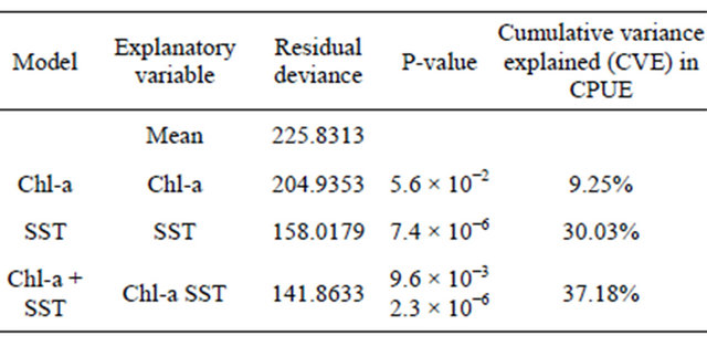
Table 2. Construction of the GLM—as each variable is added, residual deviance, the approximate AIC, and Pvalue are examined to find the best model fit.

Rug plots on the horizontal axis represent observed data points and the fitted function is shown by the thick line.
The dashed line indicates the 95% confidence bands. Both SST and Chl-a had a negative effect on skipjack CPUE. It is important to see that skipjack CPUE increases with Chl-a from 0.15 to 0.20 mg·m−3 and SST from 28.5˚C to 30.5˚C. The SST and Chl-a values outside the preferred oceanographic ranges is unclear because the reduced density of fishery data points leads to larger standard error ranges (wider confidence bands). These results confirm that the frequency of fishing sets mostly distributes within the preferred environmental conditions. Pole and line fishery tends to follow the potential fishing zone displacement. The GAM plots (rug plots) are substantially reinforced by the histogram graphs (Figure 5). From this graph, distribution of Chl-a data presented more specific and sharper than that of SST. It implies that skipjack tuna are more tolerable in physiological adaptation and temperature limit in equatorial region. Temperature limits horizontal and vertical distribution of skipjack tuna, and this varies by region and size [23]. It is more probable that skipjack tuna captured within study area have various sizes. The preferred SST range within the Bone Bay-Flores sea is higher than in subtropical waters [10,11], but it has more specific in surface Chl-a range.
3.3. Spatial Prediction of Potential Fishing Zone for Skipjack Tuna
Figure 6 shows the spatial prediction of skipjack CPUE and the potential fishing zones. The predicted CPUE for skipjack tuna present a southward displacement from

Figure 5. Generalized additive model derived effect of SST and Chl-a on nominal skipjack CPUE deviance (upper). Both independent variables are included in the GAM. Dashed lines indicate 95% confidence bands. Histogram of fishing frequency in relation to both SST and Chl-a (lower).
April (western Flores Sea around 6˚S), extending to Bone Bay in May, after which there is a highly potential fishing zones formed in Bone Bay (121˚E - 121.5˚E and 4˚S - 4.5˚S). The potential fishing zones developed when the nutrient-rich waters stimulating by the seasonal upwelling well enhanced from June to August. In July and August, the areas with relatively high skipjack CPUEs are persistently concentrated within the Bone Bay. A good feeding ground was well formed during this period and leads to significantly increase CPUE particularly in August. During the peak southeast monsoon (June-August), the potential fishing zones developed and these were accessible for fishery activities where the CPUE were highest (Figure 6).
This is clearly characterized by the development of preferred oceanographic ranges (SST and Chl-a). The predicted values lie from zero to approximately 286 fish per fishing set. The predicted CPUE map indicates that skipjack CPUE was highest in June and was consistent with the fishing data overlaid on the map (Figure 6). However, monthly mean CPUE from fishery was highest in August. This discrepancy may be as a consequence relatively wider areas of potential fishing zone in June than those in August. Fishermen capture the fish in a narrow longitudinal band and get the highest catch. Overall, the correlation of predicted and observed CPUEs pooled monthly showed a significant relationship (P < 0.01; R2 = 0.80) (Figure 7). This suggests the predicted model used in this study is consistent for predicting the potential fishing zones in the Bone Bay-Flores Sea. These findings could be as a preliminary nature of results in providing new insight into detection of potential fishing zones for skipjack tuna in equatorial region.
4. Conclusion
During the southeast monsoon particularly from June to August, the potential fishing zone for skipjack tuna in Bone Bay-Flores Sea corresponded mostly with the intensity of upwelling. The existence of upwelling during this season stimulated the enhancement of nutrient richwaters, and formed a highly biological productivity and a good feeding ground. The locations where feeding ground well developed were ultimately capable of creating potential fishing zones for skipjack. The predicted CPUE by the statistical model was significantly consistent with the observation data suggesting the spatial dynamics of potential fishing zone for skipjack tuna can be characterized and predicted using spatial signatures of both SST and Chl-a derived satellite remotely sensed data.
5. Acknowledgements
We are greatly indebted to Hildayani, Adi Jufri and Fitri Indahyani (Graduated Students, Hasanuddin University)

Figure 6. The spatial distribution of skipjack CPUE (skipjack/fishing sets) from the pole and line fishery shown as dots for April-August, 2012 overlain on the predicted CPUE derived GAM-GLM (linear model).

Figure 7. A scatter plot of pooled monthly observed against predicted skipjack CPUE values (P < 0.01, R2 = 0.80).
for all assistance in collecting the pole and line fishery data during 5 months scientific survey in Bone Bay and Flores Sea. We also appreciate the use of AQUA-MODIS SST and chlorophyll-a data sets, downloaded from the ocean color portal (http://oceancolor.gsfc.nasa.gov). This work was partly supported to MZ by the Excellent Research Based-Study Program Research Grant (Riset Unggulan Berbasis Program Studi), LP2M Hasanuddin University. This study was also partly supported to Authors by the Research of National Priority MP3EI, Dirjen Dikti, Indonesia.
REFERENCES
- A. Gordon, “The Oceanography of the Indonesian Seas and Their Throughflow,” Oceanography, Vol. 18, No.4, 2005, pp. 14-27. doi:10.5670/oceanog.2005.01
- T. Qu, Y. Du, J. Strachan, G. Meyers and J. Slingo, “Sea Surface Temperature and Its Variability in the Indonesian Region,” Oceanography, Vol. 18, No. 4, 2005, pp. 50-61. doi:10.5670/oceanog.2005.05
- J. Sprintal and T. Liu, “Ekman Mass and Heat Transport in the Indonesian Seas,” Oceanography, Vol. 18, No.4, 2005, pp. 88-97. doi:10.5670/oceanog.2005.09
- A. Mallawa, “Pemetaan Daerah Penangkapan, Hubungan Habitat Selection dan Best Fishing Ground. Bahan Ajar Program S3 Ilmu Pertanian minat Perikanan,” Program Pasca Sarjana UNHAS. Tidak Dipulikasikan, Unpublished Paper, 2009, p. 67.
- M. Zainuddin, “Skipjack Tuna In Relation To Oceanograohic Contions of Bone Bay Using Remotely Sensed Satellite Data,” Jurnal Ilmu Dan Teknologi Kelautan Tropis, Vol. 3, No. 1, 2011, pp. 82-90.
- M. Zainuddin, “Preliminary Findings on Distribution and Abundance of Flying fish in Relation to Oceanographic Conditions of Flores Sea Observed from Multi-Spectrum Satellite Images,” Asian Fisheries Science Journal, Vol. 24, No. 1, 2011, pp. 20-30.
- M. Uda, “Pulsative Fluctuation of Oceanic Fronts in Association with Tuna Fishing Ground and Fisheries,” Faculty of Marine Science and Technology, Tokai University, Vol. 7, 1973, pp. 245-265.
- A. G. Ramos, J. Santiago, P. Sangra and Canton, “An Application of Satellite-Derived Sea Surface Temperature Data to the Skipjack (Katsuwonus pelamis Linnaeus,1758) and Albacore Tuna (Thunnus alalunga Bonaterre,1788) Fisheries in the North-East Atlantic,” International Journal of Remote Sensing, Vol. 17, No. 4, 1996, pp. 749-759. doi:10.1080/01431169608949042
- P. Lehodey, M. Bertignac, J. Hampton, A. Lewis and J. Picaut, “El Niño Southern Oscillation and Tuna in the Western Pacific,” Nature, Vol. 389, 1997, pp. 715-718. doi:10.1038/39575
- H. A. Andrade and A. E. Garcia, “Skipjack Tuna in Relation to Sea Surface Temperature off the Southern Brazilian Coast,” Fisheries Oceanography, Vol. 8, No. 4, 1999, pp. 245-254. doi:10.1046/j.1365-2419.1999.00107.x
- R. Mugo, S. Saitoh, A. Nihira and T. Kuroyama, “Habitat Characteristics of Skipjack Tuna (Katsuwonus pelamis) in the Western North Pacific: A Remote Sensing Perspective,” Fisheries Oceanography, Vol. 19, No. 5, 2010, pp. 382-396. doi:10.1111/j.1365-2419.2010.00552.x
- A. Bertrand, E. Josse, P. Bach, P. Gros and L. Dagorn, “Hydrological and Trophic Characteristics of Tuna Habitat: Consequences on Tuna Distribution and Longline Catchability,” Canadian Journal of Fisheries and Aquatic Sciences, Vol. 59, No. 6, 2002, pp. 1002-1013. doi:10.1139/f02-073
- J. F. R. Gower, “A Survey of the Uses of Remote Sensing from Aircraft and Satellites in Oceanography and Hydrography,” Pacific Marine Science Report Institute of Ocean Sciences, Sidney, Vol. 72, No. 3, 1972, p. 39.
- M. Zainuddin, K. Saitoh and S. Saitoh, “Detection of Potential Fishing Ground for Albacore Tuna Using Synoptic Measurements of Ocean Color and Thermal Remote Sensing in the Northwestern North Pacific,” Geophysical Research Letters, Vol. 31, No. 20, 2004.
- M. Zainuddin, K. Saitoh and S. Saitoh, “Albacore Tuna Fishing Ground in Relation to Oceanographic Conditions of Northwestern North Pacific Using Remotely Sensed Satellite Data,” Fisheries Oceanography, Vol. 17, No. 2, 2008, pp. 61-73. doi:10.1111/j.1365-2419.2008.00461.x
- Mathsoft, “S-Plus 2000 Guide to Statistics: Data Analysis Products Division,” Vol. 2, Mathsoft Inc., Seattle, 1999, p. 638.
- P. McCullaghand and J. A. Nelder, “Generalized Linear Models,” Chapman & Hall, London, 1989, p. 532.
- A. Bertrand, E. Josse, P. Bach, P. Gros and L. Dagorn, “Hydrological and Trophic Characteristics of Tuna Habitat: Consequences on Tuna Distribution and Longline Catchability,” Canadian Journal of Fisheries and Aquatic Sciences, Vol. 59, No. 6, 2002, pp. 1002-1013. doi:10.1139/f02-073
- M. Zainuddin, H. Kiyofuji, K. Saitoh and S. Saitoh, “Using Multi-Sensor Satellite Remote Sensing and Catch Data to Detect Ocean Hot Spots for Albacore (Thunnus alalunga) in the Northwestern North Pacific,” Deep Sea Research Part II: Topical Studies in Oceanography, Vol. 53, No. 3-4, 2006, pp. 419-431. doi:10.1016/j.dsr2.2006.01.007
- S. Birowo, “The Possibility of Upwelling Occurrence in Flores Sea and Bone Bay (Text in Indonesian and abstract in English),” Oseanologi di Indonesia, Vol. 79, No. 12, 1979, pp. 1-12.
- K. Wirtky, “Physical Oceanography of Southeast Asian Waters. Naga Report 2,” Scripps Institution of Oceanography, La Jolla, 1961, p. 195.
- R. D. Susanto, A. I. Gordon and Q. Zheng, “Upwelling along the Coasts of Java and Sumatra and Its Relation to ENSO,” Geophysical Research Letter, Vol. 28, No. 5, 2001, pp. 1599-1602. doi:10.1029/2000GL011844
- P. N. Sund, M. Blackburn and F. Williams, “Tuna and Their Environment in the Pacific Ocean: A Review. Oceanogr,” Oceanography and Marine Biology: An Annual Review, Vol. 19, 1981, pp. 443-512.