Open Journal of Applied Sciences
Vol.3 No.2(2013), Article ID:33367,8 pages DOI:10.4236/ojapps.2013.32025
ROC Analysis in Radiotherapy: A TCP Model-Based Test
Department of Physics-FFCLRP, University of São Paulo, Ribeirão Preto, Brazil
Email: mairon@usp.br
Copyright © 2013 Mairon M. Santos, Ubiraci P. C. Neves. This is an open access article distributed under the Creative Commons Attribution License, which permits unrestricted use, distribution, and reproduction in any medium, provided the original work is properly cited.
Received April 4, 2013; revised May 5, 2013; accepted May 13, 2013
Keywords: Prostate Cancer; Radiotherapy; Tumour Control Probability; Hypothesis Test; ROC Curve; Dawson-Hillen Model; Monte Carlo Simulation
ABSTRACT
Several mathematical models have been proposed to describe the dynamics of irradiated cancer cells and to evaluate the tumour control probability (TCP). In this article, we propose a TCP model-based statistical test for predicting the outcome of a radiation treatment. We determine the foresight capability of prostate tumour erradication (cure) from Monte Carlo simulations of the Dawson-Hillen TCP model. We construct the receiver operating characteristic (ROC) curves of the test from the probability distributions of the fraction of remaining tumour cells for simulated experiments that evolve either to cure or non-cure. Simulations show that a similar procedure may be applicable to clinical data. Results suggest that the evaluation of tumour sizes after the treatment has started may be used for short-term prognosis.
1. Introduction
Tumour Control Probability (TCP) models have been widely used to compare different strategies in cancer therapy [1-4]. Some of these models have properties derived from multi-cellular biological systems approach and are analyzed either by continuum or cell-based models [5]. It has been shown recently that for the case of prostate cancer—and low proliferating tumours in general—diferent TCP models for radiotherapy lead practically to the same predictions regarding the TCP evolution in time [6], suggesting the use of simpler and more computationally feasible models in the clinic. However these simpler models tend to neglect the peculiar biological differences between tumours. The Monte Carlo method plays a fundamental role when one aims to include such differences into the TCP calculations.
The radiotherapy consists of depositing a certain amount of radiation dose into the tissue in order to kill the tumour cells. The dose is defined as the radiation energy deposited into the tissue per unit mass and is measured in units of gray (1 Gy = 1 Joule·kg−1). The treatment involves strategies which maximize the dose on the tumour while minimize it on the normal surrounding tissue [7]. Although the accuracy and precision of the dose have improved considerably due to technological advances [8], these are still limiting factors for a total success in radiotherapy [9,10]. Various studies have evaluated the effects of the non-uniformity of the dose deposition and heterogeneity of cancer cells in the same tumour [8,11]. Recently, the tumour control in radiation therapy was revised by Zaider and Hanin [12].
In this context, we propose a TCP model-based test for prediction of tumour erradication (cure) in radiotherapy. We obtain sampled data from Monte Carlo simulations of the two-compartment Dawson-Hillen (DH) model [1, 6]. We add a gaussian noise into the radiation dose in order to simulate the uncertainty on its deposition. Our simulations follow a particular protocol of radiation therapy for prostate cancer. A positive aspect of this procedure is that both diversity of patients and dose imprecision can be simulated. To determine the statistical power of the proposed test, we construct its receiver operating characteristic (ROC) curve from the probability distribution of the fraction of remaining tumour cells for simulated experiments that evolve either to cure or non-cure. ROC curve is an important tool which has been widely used in many research areas such as radiology [13] and signal analysis [14-16]. In a recent study [17] ROC curves were used in prediction procedures related to prostate disease.
Our study is based on simulations and a similar procedure may be applicable to clinical data. Specifically the clinical evaluation of tumour sizes may be used for shortterm prognosis in radiotherapy.
2. Monte Carlo Simulations for a TCP Model
2.1. The Dawson-Hillen TCP Model
As a generalization of the previous TCP model presented by Zaider and Minerbo [2], Dawson and Hillen developed a model [1] where the tumour cells are divided into two compartments, say active and quiescent. Cells from the quiescent compartment can migrate to the active one by an average rate  and undergo mitosis at constant rate
 , thus giving rise to two identical cells. These two cells on their turn immediately become quiescent thus repeating the cycle. The dynamics is governed by the set of equations [1]
 (1)
(1)
where  and
and  are respectively the number of cells and the mean death rates (caused by the radiation) in the active
  and quiescent
  compartments at time
 . For our purposes, it is also usefull to define
  as the total number of tumour cells (active and quiescent ones) at time
 .
.
The mean death rate is related to the survival fraction [2] in the corresponding compartment. After receiving a certain amount of radiation dose , acumulated in the time interval
 , the expected fraction of surviving cells
  in the
  compartment is given by
  well known in the literature as the Linear-Quadratic Model [18], where
  and
and ![]() are parameters related to the radiosensitivities
are parameters related to the radiosensitivities  in the
  compartment. The derivative of
  is expressed by
 (2)
(2)
so that the time evolution of the mean death rate is written as [2]
 (3)
(3)
where  is the dose rate. Since dividing cells are more sensitive to radiation
  the death rate turns to be different for each compartment. From these equations Dawson and Hillen extended the ZiderMinerbo’s approach and obtained explicit expressions for the TCP which depend on the initial number of tumour cells in each compartment [1,2].
2.2. A Monte Carlo Implementation for Sampling
Gong et al. [6] compared different TCP models regarding to clinical treatment protocols for prostate cancer. In this study, the Monte Carlo method was used as a valid approach to determine the tumour survival for one and twocompartment models.
In the present study, we propose a TCP model-based test for radiotherapy and evaluate its statistical power. For this purpose, we now describe a general Monte Carlo procedure for sampling and constructing the ROC curve of the test.
In our approach, the dynamics of tumour growth and death is governed by Equations (1), (2) and (3) of the DH two-compartment TCP model. In this way, for a time step  each cancer cell can: 1) migrate from quiescent compartment to the active one with probability
 ; 2) divide by mitosis in the active compartment with probability
 , thus originating two cells in the quiescent compartment; 3) be killed by radiation in the respective compartment with probability
  or; 4) remain unchanged otherwise. For each Monte Carlo experiment, the system evolves in time according to the above probabilistic rules. Clinically, the treatment is interrupted when the prescribed maximum dose
  is reached.
Table 1 shows a typical schedule for prostate cancer treatment used in our simulations: the nominal dose d received per fraction, the daily frequency of irradiation, the number of treatment days per week, the total number of treatment days and the corresponding nominal dose .
.
This protocol corresponds to the treatment schedule used by Parsons et al. [19] except for the number of treatment days per week. In Parsons’ protocol, no radiation dose is deposited on weekends so that such number is 5 as usual in standard treatments. Nevertheless, in our simulations the treatment is never interrupted so that the probability of tumour eradication can be continuously evaluated as function of time. In this way, statistical analysis is prevented from gaps in time if dose is deposited everyday. Naturally, such analysis can be extended to weekends off schedules.
Table 2 lists typical prostate cancer parameters used in our simulations: the initial number  of tumour cells (active and quiescent ones), the net mean rates for mitosis
  and migration
 ![]() (both ones discounted
(both ones discounted

Table 1. Treatment schedule for a prostate cancer. The patient receives 1.2 Gy twice a day until the accumulated dose reaches 76.8 Gy. The total dose settles the overall time of treatment in 32 days.

Table 2. Typical prostate cancer parameters used in the simulations [6]. First column indicates the initial number N0(0) of tumour cells (active and quiescent ones). Second column shows the net mean rates for migration (![]() ) and mitosis (μ). Third and last columns show the parameters related to the radiosensitivities for each compartment.
) and mitosis (μ). Third and last columns show the parameters related to the radiosensitivities for each compartment.
from natural death rates in the active and quiescent compartments, respectively, as in reference [3]) and the parameters  and
and ![]() related to the radiosensitivities in the
related to the radiosensitivities in the  compartment. The chosen parameters are the same ones as used by Gong et al. [6] when studying the DH two-compartment model. Prostate tumours have different radiosensitivities [20] (and thus react differently to the treatment) since cancer cells properties differ from one tumour to another and even in the same tumour. Nevertheless, cells in the same compartment of the model are considered to be identical [3].
2.3. Noise in the Absorbed Dose
During the j-th time interval  in which the tumour is irradiated at a constant dose rate
  (where
 ![]() is the j-th initial time of irradiation and
is the j-th initial time of irradiation and ![]() is the interval duration), the cumulative dose is expected to grow linearly from
is the interval duration), the cumulative dose is expected to grow linearly from  up to
up to . Although the calculation of the dose that the patient is supposed to receive has considerably improved in recent years, the clinicians still find it a limiting factor [7,21] to successfully eliminate the tumour. Indeed, the geometry of the tumour cannot be perfectly determined, the organs of the patient can move during irradiation, vascularization of the tumour is very likely to be different from one patient to another as well as between types of tumour cells and so forth. All these factors contribute to uncertainties in the effective dose deposited in the tumour.
In order to take such uncertainties into account, a gaussian noise is added into the dose d received per fraction in our Monte Carlo simulations. In this sense, the effective dose  absorbed by the tumour is sampled from a Normal distribution with mean d and variance
 , i.e.
 . Besides, the cumulative dose D is assumed to be a stochastic variable with constant probability density function
  for
for  <
<  so that its mean value is
  and its variance is given by
 . Once the absorbed dose D may be regarded as a continuous time signal, the addition of noise can be quantified in terms of the Signal to Noise Ratio (SNR), a measure used in science to evaluate the power ratio between a signal and a noise in logarithmic decibel (dB) scale. In this case SNR is calculated as
 (4)
(4)
In the Monte Carlo simulations, we use  as the irradiation time to achieve a prescribed dose d per fraction (
 as indicated in Table 1). The variance of the signal is
 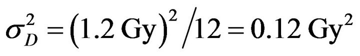 and its standard deviation is
 . Uncertainties on dose deposition are simulated by choosing
  = 0.4 Gy and
  as the standard deviations of noise. Therefore the Signal to Noise Ratios used in our simulations are
  and −10.79 dB, respectively.
3. Statistical Analysis
3.1. The Effect of Noise in the Simulations
Our statistical analysis is based on the results of a great number  of Monte Carlo simulations of the DH TCP model (see Section 2). Simulations are performed by using those parameters indicated in Tables 1 and 2. Furthermore gaussian noise is introduced in the absorbed dose as described in Section 2.3. For each simulation, tumour is irradiated during
  twice a day and this process is repeated everyday (even on weekends). Although the clinical treatment is finished when the cumulative dose reaches the prescribed value
 , each Monte Carlo experiment is let to evolve until no tumour clonogenic cell is found. Indeed, the dynamics of the model is always observed to lead to tumour eradication after a sufficiently long time. In this way, we can keep track of all events that precede the eradication.
Figure 1 compares how the cumulative dose varies with time (in simulations with ) for treatment schedules where the tumour is irradiated daily as in the present study (red line) and where no radiation dose is deposited on weekends (blue line). The small graph on the top-left corner magnifies the 10 min irradiation interval in which the absorbed dose effectively increases a variable amount
  (equals to 1.2 Gy on average). Variable growing rates are due to noise. Both plots have stair-function shapes. The widder steps in the continuous plot correspond to weekends in which no radiation dose is prescribed.
An interesting result is the influence of SNR in the time that the tumour takes to be eradicated. This effect is observed in the histograms shown in Figure 2 which present the frequency of tumour eradication as function of time for two different signal to noise ratios (
 and
and ). The quadratic term in the exponent of Equation (2) is responsible for the

Figure 1. Cumulative dose as function of time for weekends off (blue line) and weekends on (red line) treatment schedules corresponding to simulations with SNR  −1.25 dB. The small graph on the top-left corner represents the increase of the absorbed during the 10 min irradiation interval.

Figure 2. Frequency of tumour eradication as function of time. Orange histogram represents the frequency of eradication for SNR = −10.79 dB. Blue histogram corresponds to SNR = −1.25 dB.
drastic effect of radiation on tumour cells. As SNR decreases, undesirable extreme doses can eventually occur. For lower doses the cell killing is moderate but for larger ones the quadratic term becomes dominant so the expected fraction of surviving cells decays abruptely. Hence tumour tends to be eradicated earlier as SNR decreases.
3.2. The Probability of Tumour Control
Tumour control occurs if clonogenic tumour cells are absent at the end of radiation treatment. Following this concept, we define cure as tumour eradication within the provided period of treatment. Thus a simulated experiment is said to evolve to cure (if the number of tumour cells falls to zero within this period) or non-cure (otherwise). As already pointed out, the time T for clinical treatment is determined by the prescribed maximum dose . For the protocol used in our simulations (see Table 1),
  and T is the time elapsed from the beggining of the 1st day up to the end of the 32nd day. Now let
  denote the number of tumour cells in the active
 , quiescent
  or both
  compartments at time t along the k-th Monte Carlo simulation. Thus
  is the total number of tumour cells at time t in a specific experiment. The dynamics is let to evolve until the time instant
  from which the corresponding number
  of tumour cells vanishes. This means that, if the eradication time is less than or equal to the treatment time
 , the k-th experiment results in cure; otherwise
  it results in non-cure.
For the k-th experiment, tumour eradication can be evaluated at each time t by the treatment success factor , as defined in [6]:
 (5)
(5)
In other words, the success factor is null at time  if at least one tumour cell is present; otherwise, it is equal to one.
The probability  of tumour control (or simply TCP) is defined as the probability of tumour eradication (i.e., the probability of finding no tumour clonogenic cells) at time t. Numerically, this can be evaluated as the relative frequency of the essays in which tumour eradication (success) is observed at time t. As larger the sampling,
  tends to approximate to a continuous function as predicted by mean-field equations [6]. Rigorously, the relative frequency is calculated in the limit that the number M of simulations tends to infinity [6]:
 (6)
(6)
Tumour control probabilities are evaluated as functions of time for 105 Monte Carlo simulations with SNR = −1.25 dB and SNR = −10.79 dB. The resulting curves (shown in Figure 3) are monotonically increasing functions of time and resemble cumulative distributions. In fact, the probability of tumour control at time t (see Figure 3) is exactly the cumulative distribution of the frequencies of tumour eradication (see Figure 2) up to time t. On the other hand, the time derivative of  leads to the frequency of eradication as function of time. Consistently, the cumulative distribution is observed to increase earlier if SNR decreases.
3.3. ROC Curves
We propose a Monte Carlo procedure for ROC analysis. It starts with a statistical hypothesis testing. The null hypothesis  establishes that a patient undergone to radiotherapy is not cured within the treatment period (this event is referred as negative and denoted by −). The

Figure 3. Probability of tumour control as function of time for SNR = −1.25 dB (red curve) and SNR = −10.79 dB (blue curve).
alternative hypothesis H1 establishes that the patient evolves to cure within the treatment period (this event is referred as positive and denoted by +). The test statistic is chosen as the fraction  of tumour cells at some fixed time t, in the active compartment
 , quiescent one
  or both of them
 . As a decision rule for the test,
  is rejected (i.e., one concludes that patient evolves to cure) if
  is observed to be less than a chosen threshold
 ; otherwise,
  is accepted.
Let  and
and  denote the probability density functions of the statistical variable fi when hypotheses
  and
and  are supposed true, respectively (time dependence is omitted for simplicity). The sensitivity of the method can be evaluated from the knowledge of the continuous distribution of
 , as the conditional probability
  of a true positive. So sensitivity is the probability of predicting cure when the treatment in fact evolves to cure and can be expressed as
 (7)
(7)
In a analogous way, the specificity is the conditional probability  of a true negative, that is, the probability of predicting non-cure when the treatment does not evolve to cure and can be expressed as
 (8)
(8)
Therefore sensitivity and specificity can be evaluated in each compartment separately as well as in both of them. In this context, the ROC curve is the plot of  (sensitivity) versus
 in the corresponding compartment(s), obtained when the threshold
  is let to vary continuously from 0 to 1. In practice, the points of the ROC curves (for the cases i = 0, 1 or 2) can be determined from a set of critical values
 , distributed in the interval
 .
.
ROC curves are determined from the probability distributions at time t corresponding to the end of the 2nd treatment day. This time is chosen for clinical reasons. First, the tumour is expected to decrease considerably as the treatment proceeds so that actual measurement of the tumour size tends to become more difficult as time passes. Second, a clinical prediction about the patient evolution would make more sense in the beginning of the treatment. For comparison, Figure 4 illustrates the probability distributions of the fraction  of tumour cells resulting from simulations on the 2nd and 7th treatment days for experiments which evolve to cure and non-cure, separately. For each graph, the sum of the frequencies corresponding to both events (cure and non-cure) is normalized to unity. The horizontal axis is in logarithmic scale in order to avoid that the plot for the 7th day gets squeezed. As expected, smaller tumour sizes are observed on the 7th day due to the cumulative dose.
Probability distributions of the fraction of tumour cells are also dependent on the prescribed maximum dose Dman and therefore on the number of treatment days. Figure 5 presents the frequency distribution of  on the second day of treatment based on experiments which evolve to cure (red line plot shaded by orange colour) or non-cure (blue line plot) for three values of prescribed dose (Dman = 75 Gy, 85 Gy and 95 Gy). Again, the sum of the frequencies corresponding to both conditions (cure and non-cure) is normalized to unity. For smaller doses (e.g., Dman = 75 Gy), most simulations evolve to non-cure so that statistics is poor for evaluating sensitivity. On the other side, for higher doses (e.g., Dman = 95 Gy), most simulations evolve to cure so that statistics is poor for evaluating specificity. To improve statistics, we decide to choose an intermediate dose (Dman = 85 Gy) for our simulations. Indeed, distributions corresponding to the intermediate value Dman = 85 Gy show an equilibrated

Figure 4. Probability distributions of the surviving fraction f0 of tumour cells on the 2nd (right graph) and 7th (left graph) treatment days for simulations which evolve to cure (red line plot shaded by orange colour) and noncure (blue line plot), separately. The horizontal axis is on logarithmic scale for better visualization.
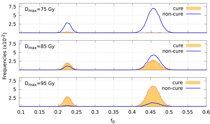
Figure 5. Frequency distribution of the surviving fraction of tumour cells f0 (on the 2nd treatment day) based on simulations which evolve to cure (red line plot shaded by orange colour) and non-cure (blue line plot). The graphs on the top, middle and bottom correspond to the prescribed doses Dmax = 75 Gy, 85 Gy and 95 Gy respectively.
number of occurences of each event (cure and non-cure) which can be seen in Figure 5.
In the present analysis, we investigate the behaviour of the variables  (total surviving fraction),
  (fraction of active cells) and
  (fraction of quiescent cells), the three of them measured at time
  corresponding to the end of the 2nd day of treatment.
The total surviving fraction can be expressed as an weighted average of tumour cells in each compartment, . In our simulations, the initial numbers of cells in the compartments are chosen to be equal
  so that
 .
.
Figure 6 shows the probability distributions for the total fraction of surviving tumour cells (bottom graph) and for the fractions of active (top graph) and quiescent (middle graph) cells. Red and blue line plots correspond to the events cure and non-cure, respectively. For each condition, the distribution of cells in the active compartment is concentrated at around fraction 0.37 whereas the distribution in the quiescent compartment presents two pronounced peaks at fractions 0.10 and 0.53 and a small peak at fraction 0.20. As a result, the distribution of  is two-peaked. As expected, the locations of both peaks in the bottom graph (at around fractions
  and
and ) are the average values of the locations of the peaks corresponding to the active and quiescent compartments.
ROC curves were determined from the probability distributions corresponding to the following values of signal to noise ratio: SNR = −1.25 dB (Figure 7) and SNR = −10.79 dB (Figure 8). The behaviour of the ROC curves for the quiescent or total compartments does not change significatively as SNR varies. For the active compartment, both sensitivity and specificity tend to increase slightly as SNR increases.
From a clinical point of view, evaluation of the frac-

Figure 6. Probability densities for the total fraction of tumour cells (bottom graph) and for the fractions of active (top graph) and quiescent (middle graph) cells. Red line plots (shaded by orange colour) and blue line plots correspond to the conditions cure and non-cure, respectively, for SNR = −1.25 dB.

Figure 7. ROC curves for the active (blue squares), quiescent (green circles) and total (red circles) compartments corresponding to SNR = −1.25 dB. The straight black line represents the hypothetic case where P(+|+) = 1 − P(−|−).

Figure 8. ROC curves for the active (blue squares), quiescent (green circles) and total (red circles) compartments corresponding to SNR = −10.79 dB. The straight black line represents the hypothetic case where P(+|+) = 1 − P(−|−).
tion  of tumour cells by medical images (at time t corresponding to the 2nd treatment day) would lead to prediction of cure (if
  were observed to be less than some threshold
 ) or non-cure (otherwise). For a good prediction, both sensitivity and specificity of the method should be as high as possible. As a criterion for determining optimum values for sensitivity and specificity (and therefore the corresponding threshold
 ), one can choose the point of ROC curve whose geometrical distance from point (1-specificity = 0, specificity = 1) is minimum. These optimum values and the corresponding critical fraction of tumour cells in each compartment (for both SNR = −1.25 dB and −10.79 dB) are presented on Table 3. For instance, according to such criterium, optimum values are achieved by adopting
  as a threshold (for SNR = −1.25 dB). In this case, if the fraction of remaining cells is estimated as smaller (greater) than 0.45, the clinician is able to predict that tumour will evolve to cure (non-cure) with 50% (62%) of certainty.
As an alternative criterium for choosing the threshold, one may require that sensitivity equals to specificity. For our simulated data, such requirement leads to the following estimatives:  (for SNR = −1.25 dB),
  (for SNR = −10.79 dB) and
 (for both SNRs).
The results exemplify this Monte Carlo approach as a viable procedure to obtain the ROC curves for radiotherapy. This ROC analysis is extensible to other TCP models and protocols.
4. Conclusion
Up to now TCP models have been analysed with regards to computational and complexity aspects [6]. In this paper we have proposed a TCP model-based test for radiotherapy and determined its ROC curve. Our Monte Carlo approach was applied to the DH TCP model (for a particular treatment protocol) and is extensible to other models and protocols. Gaussian noise was introduced in

Table 3. Sensitivities P(+|+) and specificities P(−|−) for active, quiescent and total fraction of cells and for two different Signal to Noise Ratios SNR = {−1.25, −10.79} dB.
the absorbed dose to simulate its uncertainties. The fraction of remaining tumour cells (on the 2nd radiation treatment day) was taken as a statistical variable for testing the hypothesis that tumour is not eradicated within the treatment period against the alternative hypothesis of cure. Sensitivity and specificity of the test were calculated by computational simulations for two different SNRs. Results suggest that a similar test may be applicable to clinical data. Instead of data simulated from TCP models, one can use real data to estimate the ROC curve. The evaluation of tumour sizes after the treatment has started may be used for short-term prognosis thus serving as a guide for clinician during radiotherapy. Medical images of tumour size can eventually be used to estimate the test statistic. For instance, if clinician—based on real data—knows in advance that treatment is likely to evolve to non-cure, strategies for treatment may be changed.
5. Acknowledgements
The authors acknowledge the Brazilian agency CNPq for financial support.
REFERENCES
- A. Dawson and T. Hillen, “Derivation of the Tumour Control Probability (TCP) from a Cell Cycle Model,” Computational & Mathematical Methods in Medicine, Vol. 7, No. 2-3, 2006, pp. 121-141. doi:10.1080/10273660600968937
- M. Zaider and G. N. Minerbo, “Tumour Control Probability: A Formulation Applicable to Any Temporal Protocol of Dose Delivery,” Physics in Medicine and Biology, Vol. 45, No. 2, 2000, pp. 279-293. doi:10.1088/0031-9155/45/2/303
- T. Hillen, G. De Vries, J. F. Gong and C. Finlay, “From Cell Population Models to Tumor Control Probability: Including Cell Cycle Effects,” Acta Oncologica, Vol. 49, No. 8, 2010, pp. 1315-1323. doi:10.3109/02841861003631487
- F. C. Henriquez and S. V. Castrillon, “The Use of a Mixed Poisson Model for Tumour Control Probability Computation in Non Homogeneous Irradiations,” Australasian Physical & Engineering Sciences in Medicine, Vol. 34, No. 2, 2011, pp. 267-272. doi:10.1007/s13246-011-0074-4
- H. Byrne and D. Drasdo, “Individual-Based and Continuum Models of Growing Cell Populations: A Comparison,” Journal of Mathematical Biology, Vol. 58, No. 4, 2009, pp. 657-687. doi:10.1007/s00285-008-0212-0
- J. F. Gong, M. M. Dos Santos, C. Finlay and T. Hillen, “Are More Complicated Tumour Control Probability Models Better?” Mathematical Medicine and Biology, Vol. 30, No. 1, 2011, pp. 1-19. doi:10.1093/imammb/dqr023
- R. Keinj, T. Bastogne and P. Vallois, “Multinomial Model Based Formulations of TCP and NTCP for Radiotherapy Treatment Planning,” Journal of Theoretical Biology, Vol. 279, No. 1, 2011, pp. 55-62. doi:10.1016/j.jtbi.2011.03.025
- R. Varadhan, S. K. Hui, S. Way and K. Nisi, “Assessing Prostate, Bladder and Rectal Doses during Image Guided Radiation Therapy—Need for Plan Adaptation?” Journal of Applied Clinical Medical Physics, Vol. 10, No. 3, 2009, pp. 56-74. doi:10.1120/jacmp.v10i3.2883
- J. Sykes, D. S. Brettle, D. R. Magee and D. I. Thwaites, “Investigation of Uncertainties in Image Registration of Cone Beam CT to CT on an Image-Guided Radiotherapy System,” Physics in Medicine and Biology, Vol. 54, No. 24, 2009, pp. 7263-7283. doi:10.1088/0031-9155/54/24/002
- M. Kasabasic, V. Rajevac, S. Jurkovic, A. Ivkovic, H. Sobat and D. Faj, “Influence of Daily Set-Up Errors on Dose Distribution during Pelvis Radiotherapy,” Archives of Industrial Hygiene and Toxicology, Vol. 62, No. 3, 2011, pp. 261-267. doi:10.2478/10004-1254-64-2011-2110
- R. Mehra, S. A. Tomlins, J. J. Yu, X. H. Cao, L. Wang, A. Menon, M. A. Rubin, K. J. Pienta, R. B. Shah and A. M. Chinnaiyan, “Characterization of TMPRSS2-ETS Gene Aberrations in Androgen-Independent Metastatic Prostate Cancer,” Cancer Research, Vol. 68, No. 10, 2008, pp. 3584-3590. doi:10.1158/0008-5472.CAN-07-6154
- M. Zaider and L. Hanin, “Tumor Control Probability in Radiation Treatment,” Medical Physics, Vol. 38, No. 2, 2011, pp. 574-583. doi:10.1118/1.3521406
- J. A. Hanley and B. J. McNeil, “The Meaning and Use of the Area under a Receiver Operating Characteristic (ROC) Curve,” Radiology, Vol. 143, No. 1, 1982, pp. 29-36.
- W. Tedeschi, H.-P. Müller, D. B. de Araujo, A. C. Santos, U. P. C. Neves, S. N. Ernè and O. Baffa, “Generalized Mutual Information Tests Applied to fMRI Analysis,” Physica A: Statistical Mechanics and Its Applications, Vol. 352, No. 2-4, 2005, pp. 629-644. doi:10.1016/j.physa.2004.12.065
- B. C. T. Cabella, M. J. Sturzbecher, D. B. de Araujo and U. P. C. Neves, “Generalized Relative Entropy in Functional Magnetic Resonance Imaging,” Physica A: Statistical Mechanics and Its Applications, Vol. 388, No. 1, 2009, pp. 41-50. doi:10.1016/j.physa.2008.09.029
- M. J. Sturzbecher, W. Tedeschi, B. C. T. Cabella, O. Baffa, U. P. C. Neves and D. B. de Araujo, “Nonextensive Entropy and the Extraction of Bold Spatial Information in Event-Related Functional MRI,” Physics in Medicine and Biology, Vol. 54, No. 1, 2009, pp. 161-174. doi:10.1088/0031-9155/54/1/011
- C. H. Morrell, L. J. Brant, S. Sheng and E. J. Metter, “Screening for Prostate Cancer Using Multivariate MixedEffects Models,” Journal of Applied Statistics, Vol. 39, No. 6, 2012, pp. 1151-1175. doi:10.1080/02664763.2011.644523
- W. K. Sinclair, “The Shape of Radiation Survival Curves of Mammalian Cells Cultured in Vitro,” Biophysical Aspects of Radiation Quality, Technical Reports Series (International Atomic Energy Agency), No. 58, 1966, pp. 21- 43.
- J. T. Parsons, W. Mendenhall, N. Cassisi, J. Isascs and R. R. Million, “Accelerated Hyperfractionation for Head and Neck Cancer,” International Journal of Radiation Oncology*Biology*Physics, Vol. 14, No. 5, 1988, pp. 649- 658.
- D. J. Carlson, R. D. Stewart, X. A. Li, K. Jennings, J. Z. Wang and M. Guerrero, “Comparison of in Vitro and in Vivo Alpha/Beta Ratios for Prostate Cancer,” Physics In Medicine and Biology, Vol. 49, No. 19, 2004, Article ID: 4477. doi:10.1088/0031-9155/49/19/003
- S. M. Bentzen, L. S. Constine, J. O. Deasy, A. Eisbruch, A. Jackson, L. B. Marks, R. K. Ten Haken and E. D. Yorke, “Quantitative Analyses of Normal Tissue Effects in the Clinic (Quantec): An Introduction to the Scientific Issues,” International Journal of Radiation Oncology* Biology*Physics, Vol. 76, No. 3, 2010, pp. S3-S9. doi:10.1016/j.ijrobp.2009.09.040