ABSTRACT

We study the time path of inflation and unemployment using the Blanchard treatment of the relationship between the two and taking the monetary policy condition into account. We solve the model both in continuous and discrete time and compare the results. The economic dynamics of inflation and unemployment shows that they fluctuate around their intertemporal equilibria, inflation around the growth rate of nominal money supply, respectively, and unemployment around the natural rate of unemployment. However, while the continuous-time case shows uniform and smooth fluctuation for both economic variables, in discrete time their time path is explosive and nonoscillatory. The hysteresis case shows dynamic stability and convergence for inflation and unemployment to their intertemporal equilibria both in discrete and continuous time. When inflation affects unemployment adversely the time paths of the two, both in discrete and continuous time, are dynamically unstable.

1. Introduction

The relationship between inflation and unemployment illustrated by the so called Phillips curve was first discussed by Phillips [1] in a path-breaking paper titled “The Relationship between Unemployment and the Rate of Change of Money Wage Rates in the United Kingdom, 1861-1957”. The standard treatment of the relationship between inflation and unemployment in dynamics involves the expectations-augmented Philips curve, the adaptive expectations hypothesis and the monetary policy condition. Solving the model allows studying the economic dynamics of the variables treated as functions of time. Thus, for example, we are able to find the time path and conditions for dynamic stability of actual inflation as well as of real unemployment. In studying the relationship between inflation and unemployment economists such as Phelps [2,3] have found no long-run tradeoff between these two, opposite to what the Phillips curve implies. In an influential 1968 paper titled “MoneyWage Dynamics and Labor Market Equilibrium” Phelps [4] studies the role of adaptive expectations in setting wages and prices. There he introduces the concept of the natural rate of unemployment and argues that labor market equilibrium is independent of the rate of inflation. This finding renders Keynesian theory of controlling the long-run rate of unemployment in the economy ineffective.

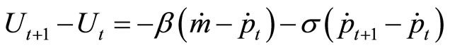
In his book Macroeconomics Blanchard [5] offers an alternative treatment of the relationship between inflation and unemployment. He incorporates in the model the natural rate of unemployment at which the actual and the expected inflation rates are equal. The rate of change of the inflation rate is proportional to the difference between the actual unemployment rate and the natural rate of unemployment.

The purpose of our paper is to study the economic dynamics and time path of inflation and unemployment from the perspective of Blanchard’s equation of the relationship between inflation and unemployment. We solve the model both in continuous and discrete time and compare the results. We discuss three cases, a simple model of Blanchard’s equation with the monetary policy condition taken into account. Then we extend the model to the hysteresis case, where inflation is adversely affected not only by unemployment but by its rate of change also. Finally, we solve the model when there is the opposite effect, that of inflation on unemployment. In studying the time path of inflation and unemployment we find that they fluctuate around their intertemporal equilibria, inflation around the growth rate of nominal money supply, respectively, and unemployment around the natural rate of unemployment. However, while the continuous-time case shows uniform and smooth fluctuation for both economic variables, in discrete time their time path is explosive and nonoscillatory. Furthermore, in the special case when present, not previous, inflation is considered, the discrete-time solution shows a non-fluctuating explosive time path. In the hysteresis case the results are identical and show dynamic stability and convergence for inflation and unemployment to their intertermporal equilibria both in discrete and continuous time. In the case when inflation affects unemployment adversely the time paths of the two both in discrete and continuous time are dynamically unstable.

The paper is organized as follows: Section 2 reveals the standard treatment of the intertemporal relationship between inflation and unemployment. In Section 3 we solve an innovative model of this relationship using Blanchard’s equation. Sections 4 and 5 extend this model to the hysteresis case and reverse influence case, respecttively. Section 6 transforms these continuous-time solutions into discrete-time results. The paper ends with concluding remarks.

2. Inflation and Unemployment: The Standard Treatment

The standard treatment of the relationship between inflation and unemployment has well been studied by mathematical economists such as Chiang [6], Pemberton and Rau [7] and Todorova [8]. The original Phillips relation shows that the rate of inflation is negatively related to the level of unemployment and positively to the expected rate of inflation such that

where is the rate of growth of the price leveli.e., the inflation rate, is the rate of unemployment and denotes the expected rate of inflation.1 Thus the expectation of higher inflation shapes the behavior of firms and individuals in a way that stimulates inflation, indeed (expecting prices to rise, they might decide to buy more presently). As people expect inflation to go down (as a result of appropriate government policies, for example), this, indeed, brings actual inflation down. This version of the Phillips relation that accounts for the expected rate of inflation is called the expectations-augmented Phillips relation. The adaptive expectations hypothesis further shows how inflationary expectations are formed. The equation

illustrates that when the actual rate of inflation exceeds the expected one, this nurtures people’s expectations so

. In the opposite case, if the actual inflation is below the expected one, this makes people believe that inflation would go down so is reduced. If the projected and the real inflation turn out to be equal, people do not expect a change in the level of inflation.

There is also the reverse effect, that of inflation on unemployment. When inflation is high for too long, this may discourage people from saving, consequently reduce aggregate investment and increase the rate of unemployment. We can write

or unemployment increases proportionally with real money where is the rate of growth of nominal money. The expression gives the rate of growth of real money, or the difference between the growth rate of nominal money and the rate of inflation

where real money is nominal money divided by the average price level in the economy. The model then becomes

(expectations-augmented Philips relation)

(adaptive expectations)

(monetary policy)

We solve this model by substituting the first equation into the second which gives

Differentiating further with respect to time,

and substituting for we obtain

where the second equation of the model implies

. Substituting this last expression for

we obtain

This is a second-order differential equation in which transforms into

or alternatively

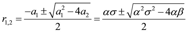
Given the properties of second-order differential equations, we have the following parameters

The coefficients and are both positive in view of the signs of the parameters. We find the equilibrium rate of expected inflation to be the particular integral

Hence, the intertemporal equilibrium of the expected rate of inflation is exactly the rate of growth of nominal money. In order to establish the time path of we need to find the characteristic roots of the differential equation which we can do using the formula

.

The time path of would depend on the particular values of the parameters. Once we find this time path we might be able to determine that of unemployment or the rate of inflation.

3. Inflation and Unemployment: An Extended Model

In his book Macroeconomics Blanchard [5] offers an alternative treatment of the relationship between inflation and unemployment. He introduces in the model the natural rate of unemployment at which the actual and the expected inflation rates are equal. The rate of change of the inflation rate is proportional to the difference between the actual unemployment rate and the natural rate of unemployment such that

Therefore, when, that is, the actual rate of unemployment exceeds the natural rate, the inflation rate decreases and when, the inflation rate increases2. The intuitive logic behind this is that in bad economic times when many people are laid off, prices tend to fall. At this point the actual unemployment would exceed the normal levels. In times of a boom in the business cycle the rate of actual unemployment would be rather low but high aggregate demand would push prices up. Blanchard’s equation reveals an important relation as it gives another way of thinking about the Phillips curve in terms of the actual and the natural unemployment rates and the change in the inflation rate. Furthermore, it introduces the natural rate of unemployment as it relates to the nonaccelerating-inflation rate of unemployment (or NAIRU), the rate of unemployment required to keep the inflation rate constant. We solve this alternative model of the relationship between inflation and unemployment by assuming that is constant and that at any given time the actual unemployment rate is determined by aggregate demand which, on its own, depends on the real value of money supply given by nominal money supply divided by the average price level. Thus unemployment is negatively related to real money supply according to the relationship

We solve by differentiating the first equation

and the second equation to obtain

We assume that the growth rate of nominal money supply is constant which could be in accordance with systematic government planning or monetary policy. The equation that obtains is identical to the monetary-policy equation introduced in the standard treatment of the Phillips curve. Combining the two results yields

which is a second-order differential equation in inflation rate. Solving the differential equation, we have, and. Hence, the particular integral is and the characteristic equation is

where and

Thus the general solution involves complex roots and takes the form

Similar to the standard model we can study the dynamic stability of actual inflation. Since, the function of inflation rate displays uniform fluctuations around the rate of growth of money supply which gives the equilibrium level of inflation.3 Since the growth rate of nominal money supply depends on government policies and changes with those, it is a moving equilibrium. Such fluctuating time path around the intertemporal equilibrium can be graphed as in Figure 1. Although the time path is not convergent, monetary policy can somewhat steer inflation and limit it within a tunnel as it fluctuates around. Given the premises of the model and the values of the parameters, a divergent time path and, therefore, an uncontrollable level of inflation are impossible.

To find the time path of unemployment as the next step we express as

and substitute it into

where the constants and have not been definitized. It follows that, similar to the inflation rate, the unemployment rate displays regular fluctuations but its intertemporal equilibrium is the natural rate of unemployment. Since this is the rate at which expected and actual inflation are equal, we can view intertemporal equilibrium as the state in which expectations coincide

with reality. Since again we have, the time path of unemployment is neither convergent, nor divergent. It follows, therefore, that with the passage of time actual unemployment cannot substantially deviate from the natural rate of unemployment.

4. The Blanchard Model: A Hysteresis System

The equation formulated by Professor Blanchard can be extended further to the so called hysteresis system. This version of the model assumes that the rate of change of the inflation rate is a decreasing function not only of the level of unemployment, but also of its rate of change. Thus even the speed with which unemployment increases will have a favourable effect on price hikes. For example, very low unemployment that increases rapidly would affect the inflation rate negatively. The inflation-unemployment model then becomes

,

Substituting for,

and differentiating with respect to gives a secondorder differential equation in

Again, nominal money supply is a stationary value for inflation rate. Here we have, and. Hence, the particular integral is and the characteristic roots are

Thus the general solution for inflation depends on the values of the characteristic roots where if, we have real roots such that

Since the constants and are positive, the roots (or their real part) turn out to be negative and the equilibrium is dynamically stable. For the unemployment rate from the first equation of the model we have

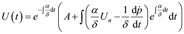
which is a first-order differential equation in unemployment with a constant coefficient and a variable term. For differential equations with a variable term and a variable coefficient of the type

where, the general solution is given by the formula. Substituting in this formula in order to solve the equation,

where and and transforming further,

where by differentiation of the inflation rate we have and, hence,

The results are consistent with our previous findings. The natural rate of unemployment again gives the intertemporal equilibrium rate for. Furthermore, a dynamically stable time path for unemployment is possible, since all exponential terms could tend to zero. The first exponential term disappears with the passage of time, while the second and the third disappear when.

5. The Effect of Inflation on Unemployment

Let us now consider a version of the extended inflation-unemployment model where there is no hysteresis, that is, inflation is unaffected by the rate of change of the unemployment level but, rather, there is the opposite effect, that of inflation on unemployment. In fact, many socially oriented economists propose maintaining some healthy levels of inflation so that to keep unemployment low. Let us assume that the rate of change of the inflation rate is a decreasing function of the level of unemployment but the unemployment rate itself is a decreasing function of both real money supply and the inflation rate. An increase in, increases aggregate demand and, therefore, lowers unemployment. Now the inflation-unemployment model takes the form

We can again analyze the time paths of and. Substituting for,

and differentiating with respect to

Again, nominal money supply is a stationary value for inflation rate. Here the parameters are, and. Hence, the particular integral is and the characteristic roots are

Thus the general solution for inflation would depend on the values of the characteristic roots. If it happens that, we have real roots . If, then we obtain complex roots for the time path of inflation. In all cases, though, we know that this time path is unstable since the parameters and are positive and the real part of the characteristic roots is also positive.

From the expression for the unemployment rate we obtain

which again gives the natural rate of unemployment as the equilibrium rate for. The general solution for unemployment by differentiation of the inflation rate is

and shows a dynamically unstable time path for unemployment.

6. Inflation and Unemployment in Discrete Time

Consider the equation formulated by Professor Blanchard in discrete time. It is equivalent to the first equation in our continuous-time inflation-unemployment model

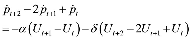
We now convert the model in a discrete-time form and solve for the time path of inflation. From the first equation of the model by further differentiation we obtained. In discrete time this involves a second difference of price on the left side, that is,

The equation in its discrete form becomes

where from the second equation of the model we have in discrete time

Thus the new model becomes

Substituting the difference term for unemployment gives a second-order difference equation in:

The equilibrium value for is

.

This result is consistent with our previous findings. The complementary function of the second-order difference equation obtained is of the type

where for the characteristic roots we have

which turn out to be complex numbers so the time path of the inflation rate must involve stepped fluctuation. Since where both and are positive constants, it must be that. Hence, the fluctuating path of inflation, given the assumptions of the model, must be explosive, as shown in Figure 2.

If we assume that the difference for unemployment is given by, that is, the increase in unemployment depends on inflation in the present, not in the previous period, the model becomes

Substituting again the difference term for unemployment results in

The equilibrium value for is

.

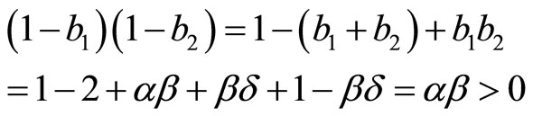
Again, the intertemporal equilibrium of inflation is the growth rate of nominal money supply. The characteristic roots are

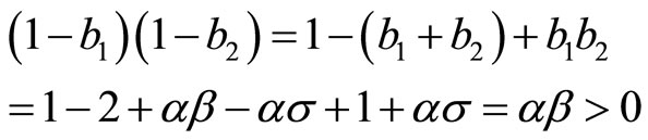
By analyzing the roots further we find

and

Since both and are positive constants, one possibility is for both roots to be negative where one is a fraction. From the second equation we also see that one

root is reciprocal of the other. Therefore, we conclude that

and

Since the absolute value of one of the roots turns out to be greater than 1, the time path of inflation is divergent and nonoscillatory. Such time path is illustrated by Figure 3.

In the special case of hysteresis the continuous-time form of the model was

We convert the model in a discrete-time form and solve for the time path of inflation. From the first equation of the model by further differentiation we have

In discrete time this involves a second difference of price on the left side and a second difference of the rate of unemployment on the right side such that

The equation in its discrete form becomes

where from the second equation of the model we have in discrete time

and also

Therefore, the equation for inflation becomes

The equilibrium value for is

which we have obtained previously. Analyzing the characteristic roots,

and

The last result implies that the characteristic roots can both be bigger than 1 or smaller than 1. This means that a convergent time path for inflation is not impossible. The condition ensures the dynamic stability of inflation. If we assume the difference for unemployment to be, the change in unemployment depends on current, not on previous, inflation. The equation of inflation is still

where

and

Substituting in the first equation,

The equilibrium value for is

.

For the characteristic roots we have

The last result again shows that a convergent time path for inflation is not impossible. However, this depends on the exact values of the parameters. Furthermore, we see that could be less than 1, given the positive values of the parameters, which also allows for convergence. If the extended inflation-unemployment model in its continuous-time form is

we modify the model in a discrete-time form

Substituting the difference term for unemployment gives a second-order difference equation in,

The equilibrium value for is

.

For the characteristic roots we have

Here since cannot be between 0 and 1, the roots cannot both be fractions. Therefore the time path of inflation would not be dynamically stable. If a different assumption is made about unemployment such as

the equation becomes

The intertemporal equilibrium for is

.

For the characteristic roots we have

Here since cannot be between 0 and 1, the roots cannot both be fractions. Therefore the time path of inflation would not be dynamically stable again.

7. Conclusion

Studying the economic dynamics of inflation and unemployment we find that their time paths show fluctuation both in continuous and discrete time. Both inflation and unemployment fluctuate around their intertemporal equilibria, inflation around the growth rate of nominal money supply, reflecting the monetary policy of the government, and unemployment around the natural rate of unemployment. However, while the continuous-time case shows uniform and smooth fluctuation for both economic variables, in discrete time their time path is explosive and nonoscillatory. Furthermore, in the special case when present, not previous, inflation is considered, the discrete-time solution shows a non-fluctuating explosive time path. In studying the hysteresis case where inflation is adversely affected not only by unemployment but by its rate of change also, the results are identical in both discrete and continuous time. The hysteresis case shows dynamic stability and convergence for inflation and unemployment to their intertemporal equilibria. Finally, in the case when inflation affects unemployment the time paths of the two both in discrete and continuous time are dynamically unstable. In all cases the dynamic stability of inflation and actual unemployment depends on the specific values of the parameters.

REFERENCES

NOTES

¹The expanded version of the Phillips relation incorporates the growth rate of money wage where the rate of inflation is the difference between the increase in wage and the increase in labor productivity, that is,. Thus inflation would result only when wage increases faster than productivity. Furthermore, wage growth is negatively related to unemployment and positively to the expected rate of inflation or where is the rate of unemployment and is the expected rate of inflation. If inflationary trends persist long enough, people start forming further inflationary expectations which shape their money-wage demands.

²Professor Blanchard [5] formulates his original equation in discrete time as.

³The time path of a general complementary function of the type depends on the sine and cosine functions as well as on the term. Since the period of the trigonometric functions is and their amplitude is 1, their graphs repeat their shapes every time the expression increases by.