Journal of Applied Mathematics and Physics, 2014, 2, 26-31
Published Online January 2014 (http://www.scirp.org/journal/jamp)
http://dx.doi.org/10.4236/jamp.2014.21005
OPEN ACCESS JAMP
Analytical Approach to Differential Equations with
Piecewise Continuous Arguments via Modified
Piecewise Variational Iteration Method
Qi Wang
School of Applied Mathematics, Guangdong University of Technology, Guangzhou, China
Received October 2013
ABSTRACT
In the present article, we apply the modified piecewise variational iteration method to obtain the approximate
analytical solutions of the differential equations with piecewise continuous arguments. This technique provides a
sequence of functions which converges to the exact solution of the problem. Moreover, this method reduces the
volume of calculations because it does not need discretization of the variables, linearization or small perturba-
tions. The results seem to show that the method is very reliable and convenient for solving such equations.
KEYWORDS
Delay Differential Equations; Piecewise Continuous Arguments; Variational Iteration Method; Approximation
1. Introduction
Differential equations with piecewise continuous arguments (EPCA) are special type of delay differential equa-
tions (DDEs). The theory of EPCA was initiated in [1,2] and developed by many authors [3-7]. These systems
have been under intensive investigation for the last twenty years. EPCA describe hybrid dynamical systems and
combine properties of both differential and difference equations. They are appeared in modeling of various
problems in real life such as biology, mechanics, and electronics. For some applications of this equation we refer
the interested reader to [1,8-10]. Several important properties of the analytic solution of EPCA as well as nu-
merical methods have been studied in [11-16].
In this paper, we consider the following two EPCA:
01
0
0
0
u'(t)au(t)au([t]),t,
u()u ,
=+≥

=

(1)
and the coupled system
23
45
x'(t )ax(t )ay([t]),
y'(t)ay(t )ax([t]),
= +

= +

(2)
with initial value
00
0
T
X()(x ,y)=
, where
i
a
01 5(i, ,,)=
are real constants and [.] denotes the greatest
integer function and
T
X(t)(x(t),y(t))=
.
In this work, we apply the modified piecewise variational iteration method (MPVIM) to systems (1) and (2) to
obtain approximate analytical solutions. The VIM gives several successive approximations by using the iteration
of the correction functional. This method was proposed by the Chinese researcher Jihuan He [17-19] as a mod-
ification of a general Lagrange multiplier method [20]. VIM is one of the non-perturbation methods that does
not require any small or large parameter. An elementary introduction of VIM is given in [21]. The main con-
cepts in VIM, such as general Lagrange multiplier, restricted variation, correction functional are explained sys-
temically. For more comprehensive survey on this method and its applications, the reader is referred to the re-
view articles [22,23] and the references therein.

Q. WANG
OPEN ACCESS JAMP
27
The VIM has been favorably applied to various kinds of linear and nonlinear problems. The main property of
the method is in flexibility and ability to solve linear and nonlinear equations accurately and conveniently. The
flexibility and adaptation provided by this method have made the method a strong candidate for approximate
analytical solutions. The VIM plays an important role in recent researches for solving various kinds of problems
(see for example [24-28] and the references therein). However, the researches on the application of VIM on
DDE are relatively fewer. As far as we know, only delay Burgers equation [29], delay logistic equation [30] and
pantograph equation [31-33] are considered. As for the analytical study of EPCA with VIM, up to now, there are
almost no results published. Therefore, we will conduct this study.
The organization of this paper is as follows. In Section 2, we simply provide the mathematical framework of
the VIM. In Section 3, we apply the modified piecewise variational iteration method on the systems (1) and (2)
after analyzing the conventional VIM and piecewise variational iteration method. Some numerical results are
given in Section 4. Finally, in Section 5, a brief conclusion is provided.
2. He’s Variational Iteration Method
In this section, we introduce the basic idea underlying the VIM for solving nonlinear equations. Consider the
general differential equation
LuNug(x ),+=
(3)
where
L
and
N
are linear and nonlinear operators, respectively, and
g( x)
is the inhomogeneous term. In
VIM, a correction functional for (3) can be written as

10
xn
nn n
u(x)u (x)(s)[Lu(s)Nu(s)g(s)]ds, λ
+
=+ +−
∫
(4)
where
λ
is a general Lagrange’s multiplier, which can be identified optimally via integration by parts and the
variational theory, and

n
u
denotes the restricted variation, i.e.

0
n
u δ
=
. It is to be noted that the Lagrange
multiplier
λ
can be a constant or a function. After determining the Lagrange multiplier
λ
, an iteration for-
mula, without restricted variation, should be used for the determination of the successive approximations
1n
u (x)
+
of the solution
u(x )
. The zeroth approximation
0
u
can be selected freely. Consequently, the solu-
tion is given by
n
n
u( x )lim u( x )
→∞
=
(5)
3. The Application of VIM
In this section the application of VIM is discussed for solving systems (1) and (2).
3.1. System (1)
We consider system (1), according to the VIM, the correction function is given by
( )
11
0
n
t'nn
nn
u(t)u(t)(s)u (s)au (s)au([s])ds. λ
+
=+ −−
∫
(6)
To find the optimal value of
λ
we have
10
n
t'
nn
u(t)u (t)(s)u(s)ds, δδ δλ
+
= +
∫
(7)
that results
( )
10
1
t
n nn
st
u(t)u (t)'(s)u(s)ds. δλ δδλ
+=
=+−
∫
(8)
Thus we have the following stationary conditions
1| 0
0
st
st
,
'( s ).
λ
λ
=
=
+=


=


(9)
This in turn gives
1 λ = −
. So we obtain the following iteration formula
( )
1 01
0
n
t'
nnn n
u(t)u (t)u(s)au(s)au([s])ds,
+
=− −−
∫
(10)

Q. WANG
OPEN ACCESS JAMP
28
and the approximation solution is given by
1n
n
u(t )limu(t )
+
→∞
=
. (11)
During the process of computation, the greatest integer function [.] causes us many problems. To overcome
them, we recall a modified VIM: the piecewise variational iteration method (PVIM), which was introduced by
Geng [34,35]. In PVIM, the interval
0[,X]
is divided into some equal subintervals, then the
i
n
-order ap-
proximation
i
i,n
u (x)
are obtained on these subintervals. Following this way, we introduce the modified piece-
wise variational iteration method (MPVIM). In our method, the interval
0[, )∞
is divided into lots of subin-
tervals
1[k,k)+
with unit length, where
kN∈
.
On the interval
01[ ,]
, let
( )
11101011 1
0
t'
,n ,,n,n,n
u(t)u(t)u (s)au (s)au([s])ds,
+
=− −−
∫
10
0
,
u(t)u(),=
(12)
where
01t[ ,]∈
. Then we can obtain the
1
n
-order approximation
1
1,n
u (t)
on
01[,]
.
On the interval
12[,]
, let
( )
212020212
0
t'
,n ,,n,n,n
u(t)u(t)u (s)au (s)au ([s])ds,
+
=− −−
∫
1
20 1
1
, ,n
u(t)u().=
(13)
The integration in (13) can be computed in
01[ ,]
and
1[ ,t]
, respectively. Then the
2
n
-order approxima-
tion
2
2,n
u (t)
on
12[,]
can be obtained.
In a similar way, on the interval
1[k ,k]−
,
34k ,,=
let
( )
100 1
0
t'
k,nk,k,nk,nk,n
u(t)u(t)u (s)au (s)au ([s])ds,
+
=−−−
∫
1
01
1
k
k ,k,n
u(t)u( k).
−
−
= −
(14)
The integration in (14) can be computed in a series of subintervals:
01[,]
,
12[ ,],,
1[k ,t]−
. Then we can
obtain the
k
n
-order approximation
k
k ,n
u (t)
on
1[k ,k]−
.
Therefore, according to (12)-(14), the approximation of (1) on the entire interval
0[, )∞
can be obtained.
3.2. System (2)
According to VIM, the iteration formula for (2) can be constructed as follows
( )
1 23
0
n
t'
nnn n
x(t)x (t)x(s)ax (s)ay ([s])ds,
+
=−−−
∫
( )
1 45
0
n
t'
nnn n
y(t)y(t)y(s)ay (s)ax ([s])ds.
+
=− −−
∫
(15)
Similar to Subsection 3.1, in view of MPVIM we have the following formulas.
On the interval
01[ ,]
, let
( )
111012 131
0
t'
,n ,,n,n,n
x(t)x (t)x(s)ax (s)ay ([s])ds,
+=−−−
∫
( )
11101415 1
0
t'
,n ,,n,n,n
y(t)y(t)y (s)ay (s)ax ([s])ds,
+
=− −−
∫
10
0
,
x(t)x(),=
10
0
,
y(t )y().=
Then we can obtain the
1
n
-order approximation
1
1,n
X (t)
on
01[,]
, where
T
X(t) (x(t),y(t))=
.
On the interval
12[,]
, let
( )
212022 232
0
t'
,n ,,n,n,n
x(t)x (t)x (s) ax (s) ay([s])ds,
+
=− −−
∫
( )
21202425 2
0
t'
,n ,,n,n,n
y(t)y (t)y (s) ay(s) ax ([s])ds,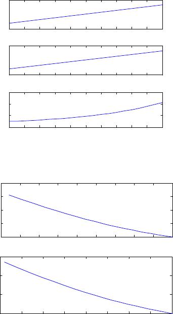
+
=− −−
∫

Q. WANG
OPEN ACCESS JAMP
29
1
20 1
1
, ,n
x(t )x(),=
1
20 1
1
, ,n
y(t )y().=
Then we can obtain the
2
n
-order approximation
2
2,n
X (t)
on
12[,]
.
Similarly, on the interval
1[k ,k]−
,
34k,,=
let
( )
102 3
0
t'
k,nk,k,nk,nk,n
x(t)x (t)x(s) ax(s) ay([s])ds,
+
=−−−
∫
( )
104 5
0
t'
k,nk,k,nk,nk,n
y(t)y(t)y(s) ay(s) ax ([s])ds,
+
=− −−
∫
1
01
1
k
k ,k,n
x(t)x( k),
−
−
= −
1
01
1
k
k ,k,n
y(t)y(k).
−
−
= −
Then we can obtain the
k
n
-order approximation
k
k ,n
X (t)
on
1[k ,k]−
.
Therefore, according to (16)-(18), the approximation of coupled system (2) on the entire interval
0[, )∞
can
be obtained.
4. Results and Discussion
In this section, we apply the MPVIM presented in Section 3 and the classical
θ
-methods to two concrete EPCA.
Numerical results show that the MPVIM is very effective.
For (1), we choose
0
2a=
,
11a= −
and
01u=
. According to (12)-(14), taking
3k=
and
5
i
n=
,
1i, ,k.=
We can obtain the approximations of (1) on
03[,]
. The numerical results are depicted in Figure 1.
This figure shows the comparison of approximation obtained by using the present method with the exact solu-
tion and the numerical solution. Moreover, for (2), we choose
2
1a=
,
3
2a= −
,
4
2a=
,
5
1a= −
and
00
1xy= =
. In Fig ure 2 we compare the 5th-order approximation of MPVIM with the numerical solution.
Figure 1. A comparison of the results of the exact solution (upper), the 5th-order MPVIM solution (middle) and the
numerical solution (lower) with θ = 0.6 and m = 20 to (1).
Figure 2. A comparison of the results of the 5th-order MPVIM solution (upper) and the numerical solution (lower)
with θ = 0.3 and m = 20 to (2).
00.1 0.20.3 0.40.5 0.6 0.70.8 0.9 1
0
5
time t
u(t )
00.1 0.20.3 0.40.5 0.6 0.70.8 0.91
0
5
time t
u
n
(t)
00.1 0.20.3 0.40.5 0.6 0.70.8 0.91
0
2
4
6
time t
u
n
-0.8 -0.6 -0.4 -0.200.2 0.4 0.6 0.81
1
2
3
4
5
x
n
(t)
y
n
(t)
-0.6 -0.4 -0.2 00.2 0.4 0.6 0.8 1
1
2
3
4
x
n
y
n

Q. WANG
OPEN ACCESS JAMP
30
The above numerical examples demonstrate that the present method is quite effective and simple.
5. Conclusions
An efficient algorithm based on the VIM has been successfully applied to the EPCA. As can be seen from the
numerical results, implementing only a few steps in the MPVIM, the approximate analytical solutions with high
accuracy can be obtained.
It can be concluded that the MPVIM is a powerful and promising tool for solving such kinds of delay diffe-
rential equations. This method can also be extended to the EPCA of the advanced type and mixed type, which
are our future research issues.
Acknowledgements
The author would like to thank the reviewers for his/her hard work. In addition, we thank Professor Fazhan
Geng for his helpful assistance.
REFERENCES
[1] S. Busenberg and K. L. Cooke, “Models of Vertically Transmitted Diseases with Sequential-Continuous Dynamics, Nonlinear
Phenomena in Mathematical Sciences,” In: V. Lakshmikantham, Ed., Academic Press, New York, 1982, pp. 179-187.
[2] K. L. Cooke and J. Wiener, “Retarded Differential Equations with Piecewise Constant Delays,” Journal of Mathematical Anal-
ysis and Applications, Vol. 99, 1984, pp. 265-297. http://dx.doi.org/10.1016/0022-247X(84)90248-8
[3] Y. K. Huang, “A Nonlinear Equation with Piecewise Constant Argument,” Applied Analysis, Vol. 33, 1989, pp. 183-190.
http://dx.doi.org/10.1080/00036818908839871
[4] J. L. Hong, R. Obayab and A. Sanzb, “Almost Periodic Type Solutions of Some Differential Equations with Piecewise Con-
stant Argument,” Nonlinear Analysis, Vol. 45, 2001, pp. 661-688. http://dx.doi.org/10.1016/S0362-546X(98)00296-X
[5] L. Dai and M. C. Singh, “A New Approach with Piecewise Constant Arguments to Approximate and Numerical Solutions of
Oscillatory Problems,” Journal of Sound and Vibration, Vol. 263, 2003, pp. 535-548.
http://dx.doi.org/10.1016/S0022-460X(02)01065-9
[6] G. Papaschinopoulos, G. Stefanidou and P. Efraimidis, “Existence, Uniqueness and Asymptotic Behavior of the Solutions of a
Fuzzy Differential Equation with Piecewise Constant Argument,” Information Science, Vol. 177, 2007, pp. 3855-3870.
http://dx.doi.org/10.1016/j.ins.2007.03.006
[7] M. Pinto, “Asymptotic Equivalence of Nonlinear and Quasi Linear Differential Equations with Piecewise Constant Arguments,”
Mathematical and Computer Modelling, Vol. 49, 2009, pp. 1750-1758. http://dx.doi.org/10.1016/j.mcm.2008.10.001
[8] L. Dai and M. C. Singh, “On Oscillatory Motion of Spring-mass Systems Subjected to Piecewise Constant Forces,” Journal of
Sound and Vibration, Vol. 173, 1994, pp. 217-232. http://dx.doi.org/10.1006/jsvi.1994.1227
[9] N. M. Murad and A. Celeste, “Linear and Nonlinear Characterization of Loading Systems Under Piecewise Discontinuous
Disturbances Voltage: Analytical and Numerical Approaches,” Proceedings of International Conference on Power Electronics
Systems and Applications, November 2004, pp. 291-297.
[10] J. Wiener and V. Lakshmikantham, “A Damped Oscillator with Piecewise Constant Time Del ay,” Nonlinear Studies, Vol. 1,
2000, pp. 78-84.
[11] R. Yuan, “On Favard’s Theorems,” Journal of Differential Equations, Vol. 249, 2010, pp. 1884-1916.
http://dx.doi.org/10.1016/j.jde.2010.07.014
[12] E. Ait Dads and L. Lhachimi, “Pseudo Almost Periodic Solutions for Equation with Piecewise Constant Argument,” Journal of
Computational and Applied Mathematics, Vol. 371, 2010, pp. 842-854. http://dx.doi.org/10.1016/j.jmaa.2010.06.032
[13] M. U. Akhmet, D. Arugaslanc and E. Y1lmaz, “Method of Lyapunov Functions for Differential Equations with Piecewise Con-
stant Delay,” Journal of Computational and Applied Mathematics, Vol. 235, 2011, pp. 4554-4560.
http://dx.doi.org/10.1016/j.cam.2010.02.043
[14] M. Z. Liu, M. H. Song and Z. W. Yang, “Stability of Runge-Kutta Methods in the Numerical Solution of Equation
u'(t)=au(t)+a0u([t]),” Journal of Computational and Applied Mathematics, Vol. 166, 2004, pp. 361-370.
http://dx.doi.org/10.1016/j.cam.2003.04.002
[15] W. J. Lv, Z. W. Yang and M. Z. Liu, “Stability of Runge-Kutta Methods for the Alternately Advanced and Retarded Differen-
tial Equations with Piecewise Continuous Arguments,” Computers & Mathematics with Applications, Vol. 54, 2007, pp. 326-
335. http://dx.doi.org/10.1016/j.camwa.2006.07.018
[16] M. Z. Liu, J. F. Gao and Z. W. Yang, “Preservation of Oscillations of the Runge-Kutta Method for Equation
x'(t)+ax(t)+a1x([t-1])=0,” Computers & Mathematics with Applications, Vol. 58, 2009, pp. 1113-1125.

Q. WANG
OPEN ACCESS JAMP
31
http://dx.doi.org/10.1016/j.camwa.2009.07.030
[17] J. H. He, “Variational Iteration Method for Delay Differential Equations,” Communications in Nonlinear Science and Numeri-
cal Simulation, Vol. 2, 1997, pp. 235-236. http://dx.doi.org/10.1016/S1007-5704(97)90008-3
[18] J. H. He, “Approximate Solution of Nonlinear Differential Equations with Convolution Product Non-Linearities,” Computer
Methods in Applied Mechanics and Engineering, Vol. 167, 1998, pp. 69-73. http://dx.doi.org/10.1016/S0045-7825(98)00109-1
[19] J. H. He, “Variational Iteration Method for Autonomous Ordinary Differential Systems,” Applied Mathematics and Computa-
tion, Vol. 114, 2000, pp. 115-123. http://dx.doi.org/10.1016/S0096-3003(99)00104-6
[20] M. Inokuti, H. Sekine and T. Mura, “General Use of the Lagrange Multiplier in Non-linear Mathematical Physics,” In: Varia-
tional Methods in the Mechanics of Solids, Pergamon Press, Oxford, 1978, pp. 156-162.
[21] J. H. He, “Variational Iteration Method-Some Recent Results and New Interpretation,” Journal of Computational and Applied
Mathematics, Vol. 207, 2007, pp. 3-17. http://dx.doi.org/10.1016/j.cam.2006.07.009
[22] J. H. He and X. H. Wu, “Variational Iteration Method: New Development and Applications,” Computers & Mathematics with
Applications, Vol. 54, 2007, pp. 881-894. http://dx.doi.org/10.1016/j.camwa.2006.12.083
[23] J. H. He, G. C. Wu and F. Austin, “The Variational Iteration Method Which Should Be Followed,” Nonlinear Science Letters A,
Vol. 1, 2010, pp. 1-30.
[24] G. C. Wu, “A Fractional Variational Iteration Method for Solving Fractional Nonlinear Differential Equations,” Computers &
Mathematics with Applications, Vol. 61, 2011, pp. 2186-2190. http://dx.doi.org/10.1016/j.camwa.2010.09.010
[25] J. F. Lu, “An Analytical Approach to the Fornberg-Whitham Type Equations by Using the Variational Iteration Method,”
Computers & Mathematics with Applications, Vol. 61, 2011, pp. 2010-2013. http://dx.doi.org/10.1016/j.camwa.2010.08.052
[26] M. M. Khader, “Numerical and Theoretical Treatment for Solving Linear and Nonlinear Delay Differential Equations Using
Variational Iteration Method,” Arab Journal of Mathematical Sciences, Vol. 19, No. 2, 2013, pp. 243-256.
http://dx.doi.org/10.1016/j.ajmsc.2012.09.004
[27] G. Yang and R. Y. Chen, “Choice of an Optimal Initial Solution for a Wave Equation in the Variational Iteration Method,”
Computers & Mathematics with Applications, Vol. 61, 2011, pp. 2053-2057. http://dx.doi.org/10.1016/j.camwa.2010.08.068
[28] A. F. Elsayed, “Comparison between Variational Iteration Method and Homotopy Perturbation Method for Thermal Diffusion
and Diffusion Thermo Effects of Thixotropic Fluid through Biological Tissues with Laser Radiation Existence,” Applied Ma-
thematical Modelling, Vol. 37, no.6, 2013, pp. 3660-3673. http://dx.doi.org/10.1016/j.apm.2012.07.016
[29] E. S. Fahmy, H. A. Abdusalam and K. R. Raslan, “On the Solutions of the Time-delayed Burgers Equation,” Nonlinear Analy-
sis, Vol. 69, 2008, pp. 4775-4786. http://dx.doi.org/10.1016/j.na.2007.11.027
[30] M. Dehghan and R. Salehi, “Solution of a Nonlinear Time-delay Model in Biology via Semi-analytical Approaches,” Computer
Physics Communications, Vol. 181, 2010, pp. 1255-1265. http://dx.doi.org/10.1016/j.cpc.2010.03.014
[31] Z. H. Yu, “Variational Iteration Method for Solving the Multi-Pantograph Delay Equation,” Physical Letter A, Vol. 372, 2008,
pp. 6475-6479. http://dx.doi.org/10.1016/j.physleta.2008.09.013
[32] A. Saadatmandi and M. Dehghan, “Variational Iteration Method for Solving a Generalized Pantograph Equation,” Computers
& Mathematics with Applications, Vol. 58, 2009, pp. 2190-2196. http://dx.doi.org/10.1016/j.camwa.2009.03.017
[33] X. M. Chen and L. J. Wang, “The Variational Iteration Method for Solving a Neutral Functional-Differential Equation with
Proportional Delays,” Computers & Mathematics with Applications, Vol. 59, 2010, pp. 2696-2702.
http://dx.doi.org/10.1016/j.camwa.2010.01.037
[34] F. Z. Geng, Y. Z. Lin and M. G. Cui, “A Piecewise Variational Iteration Method for Riccati Differential Equations,” Computers
& Mathematics with Applications, Vol. 58, 2009, pp. 2518-2522. http://dx.doi.org/10.1016/j.camwa.2009.03.063
[35] F. Z. Geng, “A Piecewise Variational Iteration Method for Treating a Nonlinear Oscillator of a Mass Attached to a Stretched
Elastic Wire,” Computers & Mathematics with Applications, Vol. 62, 2011, pp. 1641-1644.
http://dx.doi.org/10.1016/j.camwa.2011.05.004