H. GOTO, Y. MATSUOKA
304
adjustment of labor as follows:
1
0 as .
2
HH
s
λ
(6)
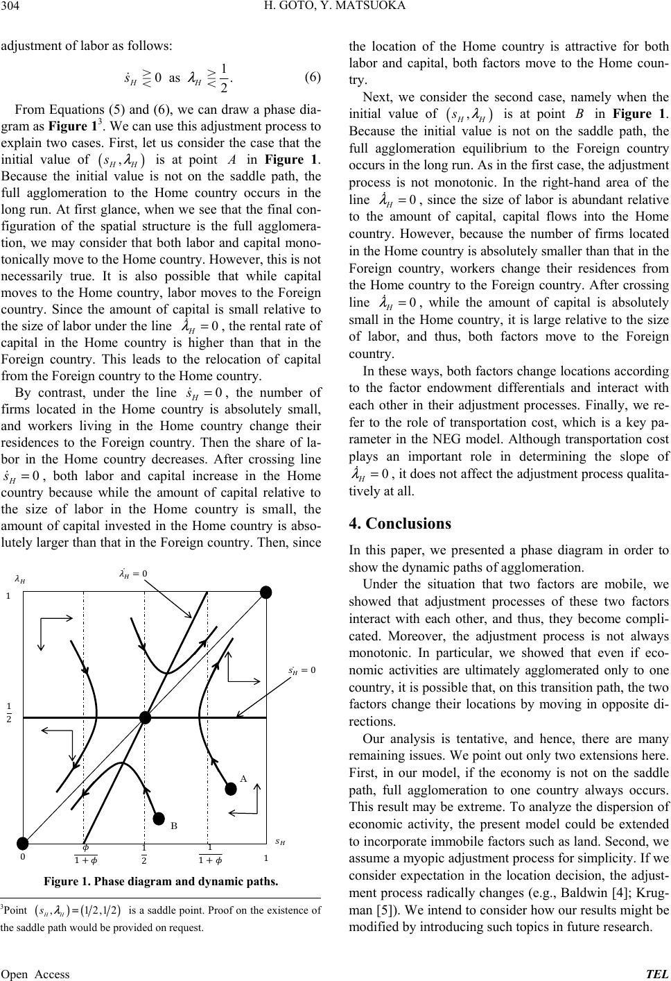
From Equations (5) and (6), we can draw a phase dia-
gram as Figure 13. We can use this adjustment process to
explain two cases. First, let us consider the case that the
initial value of
(
is at point
)
,
HH
s
λ
in Figure 1.
Because the initial value is not on the saddle path, the
full agglomeration to the Home country occurs in the
long run. At first glance, when we see that the final con-
figuration of the spatial structure is the full agglomera-
tion, we may consider that both labor and capital mono-
tonically move to the Home country. However, this is not
necessarily true. It is also possible that while capital
moves to the Home country, labor moves to the Foreign
country. Since the amount of capital is small relative to
the size of labor under the line , the rental rate of
capital in the Home country is higher than that in the
Foreign country. This leads to the relocation of capital
from the Foreign country to th e Home country.
0
H
λ
=
By contrast, under the line , the number of
firms located in the Home country is absolutely small,
and workers living in the Home country change their
residences to the Foreign country. Then the share of la-
bor in the Home country decreases. After crossing line
, both labor and capital increase in the Home
country because while the amount of capital relative to
the size of labor in the Home country is small, the
amount of capital invested in the Home country is abso-
lutely larger than that in the Foreign country. Th en, since
0
H
s=
0
H
s=
1
1
1
1
2
0
0
1
1
0
1
2
B
Figure 1. Phase diagram and dynamic paths.
the location of the Home country is attractive for both
labor and capital, both factors move to the Home coun-
try.
Next, we consider the second case, namely when the
initial value of
(
is at point in Figure 1.
Because the initial value is not on the saddle path, the
full agglomeration equilibrium to the Foreign country
occurs in the long run. As in the first case, the adju stment
process is not monotonic. In the right-hand area of the
line , since the size of labor is abundant relative
to the amount of capital, capital flows into the Home
country. However, because the number of firms located
in the Home country is absolutely smaller than that in the
Foreign country, workers change their residences from
the Home country to the Foreign country. After crossing
line , while the amount of capital is absolutely
small in the Home country, it is large relative to the size
of labor, and thus, both factors move to the Foreign
country.
)
,
HH
s
λ
B
0
H
λ
=
0
H
λ
=
In these ways, both factors change locations according
to the factor endowment differentials and interact with
each other in their adjustment processes. Finally, we re-
fer to the role of transportation cost, which is a key pa-
rameter in the NEG model. Although transportation cost
plays an important role in determining the slope of
, it does not affect the adjustment process qualita-
tively at all.
0
H
λ
=
4. Conclusions
In this paper, we presented a phase diagram in order to
show the dynamic pat hs o f agglome ra t ion.
Under the situation that two factors are mobile, we
showed that adjustment processes of these two factors
interact with each other, and thus, they become compli-
cated. Moreover, the adjustment process is not always
monotonic. In particular, we showed that even if eco-
nomic activities are ultimately agglomerated only to one
country, it is possible th at, on this tran sition path , the two
factors change their locations by moving in opposite di-
rections.
Our analysis is tentative, and hence, there are many
remaining issues. We point out only two extensions here.
First, in our model, if the economy is not on the saddle
path, full agglomeration to one country always occurs.
This result may be extreme. To analyze the dispersion of
economic activity, the present model could be extended
to incorporate immobile factors such as land. Second, we
assume a myopic adjustment process for simplicity. If we
consider expectation in the location decision, the adjust-
ment process radically changes (e.g., Baldwin [4]; Krug-
man [5]). We intend to consider how our results might be
modified by introducing such topics in future research.
3Point
()(
,12,1
HH
s
λ
=
)
2
is a saddle point. Proof on the existence o
the saddle path would be provided on request.
Open Access TEL