 Engineering, 2013, 5, 975-988 Published Online December 2013 (http://www.scirp.org/journal/eng) http://dx.doi.org/10.4236/eng.2013.512119 Open Access ENG Numeric Solution of the Fokker-Planck-Kolmogorov Equation Claudio Floris Department of Civil and Environmental Engineering, Politecnico di Milano, Milano, Italy Email: claudio.floris@polimi.it Received March 12, 2013; revised April 12, 2013; accepted April 19, 2013 Copyright © 2013 Claudio Floris et al. This is an open access article distributed under the Creative Commons Attribution License, which permits unrestricted use, distribution, and reproduction in any medium, provided the original work is properly cited. ABSTRACT The solution of an n-dimensional stochastic differential equation driven by Gaussian white noises is a Markov vector. In this way, the transition joint probability density function (JPDF) of this vector is given by a deterministic parabolic par- tial differential equation, the so-called Fokker-Planck-Kolmogorov (FPK) equation. There exist few exact solutions of this equation so that the analyst must resort to approximate or numerical procedures. The finite element method (FE) is among the latter, and is reviewed in this paper. Suitable computer codes are written for the two fundamental versions of the FE method, the Bubnov-Galerkin and the Petrov-Galerkin method. In order to reduce the computational effort, which is to reduce the number of nodal points, the following refinements to the method are proposed: 1) exponential (Gaussian) weighting functions different from the shape functions are tested; 2) quadratic and cubic splines are used to interpolate the nodal values that are known in a limited number of points. In the applications, the transient state is stud- ied for first order systems only, while for second order systems, the steady-state JPDF is determined, and it is compared with exact solutions or with simulative solutions: a very good agreement is found. Keywords: Stochastic Differential Equations; Markov Vectors; Fokker-Planck-Kolmogorov Equation; Finite Element Numeric Solution; Modified Hermite Weighting Functions; Spline Interpolation 1. Introduction It is widely recognized that many types of agencies act- ing on engineering structures and equipments have ran- dom characteristics. This is the case of earthquakes, wind load, wave load, electric current in a circuit, and so on. Thus, these agencies are to be described by means of the theory of stochastic processes. Moreover, in some cases, the structural properties themselves are uncertain, and must be considered as stochastic processes, which gives raise to a multiplicative or parametric excitation. In this way, the differential equations that govern the response become stochastic differential equations. If the differential equations that govern the response are nonlinear or the excitation is parametric or both, the random response analysis is not an easy task, and mathe- matically exact solutions for the statistical characteriza- tion are not available in many cases. However, if the ex- citations are Gaussian white noise (WN) random proc- esses, the system response is a vector Markov process, too: see [1-3]. If the initial state of a Markov process is known, then the joint probability density function (JPDF) of the states characterizes completely the stochastic process. The JPDF is the solution of a parabolic partial differential equation (PDE), the so-called Fokker-Planck-Kolmo- gorov (FPK) equation. This equation depends on time and on the actual values of the system states. However, if the system is damped and stable, a stationary state exists, which is characterized by the stationary JPDF p(x), which does not depend on time. The FPK equation loses the dependence on time, and is called reduced FPK equa- tion. A wide treatment of it can be found in [3,4]. The severe limitations of the FPK equation approach resides in that exact analytical solutions are available in a restricted number of cases, and mostly in the steady state. In the transient state, analytical solutions were obtained for scalar systems only: the reader is referred to [4]. Along the years, much theoretical work has been done in order to solve the reduced FPK equation: [5-27]. Not- withstanding the considerable progress in this matter, two serious flaws remain: 1) in the case of multiplicative excitations, for the FPK equation to be solvable, restric- tive relationships among the system parameters and the  C. FLORIS 976 spectral densities of the excitations must be satisfied, and such requirements are rarely encountered in practical cases; 2) in several cases, no analytical solutions have been found, among the case of oscillators with a generic nonlinear damping mechanism. For these reasons, the sixties numerical schemes of solution have been developed parallelly to the theoretical studies. These methods are: weighted residual method, eigenfunction expansion, finite differences, variational principles, and finite element (FE) method. In the weighted residual method [28-33], the functional form of the JPDF is chosen a priori: a mixture of Gaus- sian functions or the exponential of a polynomial in the state variables is the most usual choice in both unknown coefficients’ appearance. The approximate form of the JPDF cannot satisfy the FPK equation exactly so that a residual error arises. It is imposed that the projection of this into a set of weighting functions vanishes. In this way, a system of equations in the unknown coefficients is obtained, and it must be solved. Muscolino, Ricciardi and Vasta’s method [29] is notable as it gives raise to an expression of the JPDF in which the coefficients are lin- ear functions of the response statistical moments. In the eigenfunction expansion method [34-38], the non-stationary JPDF of the system states is expressed as a truncated series of orthogonal functions, which are functions that form a complete orthonormal basis in a Hilbert space [39]. If the eigenfunctions of the FPK equation were available in all cases, this representation would be exact, but in general they are not known, and their computation even in an approximate numerical form is often cumbersome. Thus, the different authors adopt different strategies: in [35,38], the orthogonal func- tions are chosen a priori, and in order to determine the coefficients of the series, the weighted residual method is used. In [34,36,37], a perturbative approach is used. Roberts use the finite difference method [40] to solve the FPK equation for the one-dimensional PDF of the energy envelope. In other words, there is only a spatial variable beyond the time variable, which is a limitation. In [41], two types of variational approaches are pre- sented, both of which are aimed at finding approximate values of the non-zero eigenvalues of the FPK operator (the first eigenvalue is zero, and it corresponds to the steady state PDF). The former one constructs an approxi- mate Hermitian operator, and the other is based on a perturbation expansion. The applications are confined to the steady state. In [42], the variational approach gives raise to an iterative procedure. The applications regard the transient state of scalar systems. The approximate solution of PDE’s by means of the finite element method (FE) is a classic topics in numeric mathematics (e.g. see [43]). Probably, Bergman and Heinrich [44-46] were the first who applied this method in the field of stochastic dynamics. In the above cited references, they did not analyze the FPK equation but the Pontriagin-Vitt equation in the moments of the first pas- sage time of a level from the displacement X of a second order oscillator (as regards the Pontriagin-Vitt equation see [3], Chap. 8); however, the principles are the same. Then, the FE method was applied to the FPK equation: [47-54]. Differently from the weighted residual method in which the transition JPDF of the state vector has the same approximate form in the whole state space, in the FE method, the state space is discretized into ele- ments inside which the JPDF varies according to the shape or trial functions that have been selected previ- ously, and depending on the nodal values (see later). In [47-54], linear shape functions are used, which insure C0 continuity only. Vice versa, as the FPK equation Equa- tions (6) and (7) contains second derivatives, it would require C1 continuity. The problem is overcomed by combining the FE method with the weighted residual method: the residual error is made orthogonal to a weight function in such a way that the coefficients of a linear system in the nodal values are computed. Fundamentally, there are two versions of the FE method for solving the FPK equation: the Bubnov-Galerkin and the Petrov- Galerkin method. In the former, the weighting functions are equal to the trial functions. Vice versa, in the latter, weighting and trial functions are different, in general the weighting functions being non linear. This version is be- lieved more suitable for convective problems [44,45,49, 52]. However, in the steady state, that is when solving the reduced FPK equation, there is no diffusion of pro- bability. With the exception of [49,52,53] in the above mentioned references, the applications regard the steady state because of the charge for computation. Some improve- ments of the method were proposed: in [51], an adaptive grid generation is used; in [53], a multi-scale FE method is fitted to the present problem; in [54], the solution is improved by means of a local hp-refinement of the mesh. The present paper is organized as follows: Sec. 2 is devoted to the FPK equation. Sec. 3 treats the FE method for solving the FPK equation: first, its theoretical deriva- tion is reviewed, and some topics are discussed. In detail, it is shown that: 1) to interpolate the nodal, values with splines of degree higher than those of the shape functions may improve the solution substantially; 2) in some cases the use of weighting functions different from the shape functions yields a notable computing time saving. The last two sections are devoted to the applications and con- clusions respectively. In order to contain the computing time, the transient state is studied for first order systems only, while for second order systems the steady-state JPDF is determined. Open Access ENG  C. FLORIS 977 2. The Fokker-Planck-Kolmogorov Equation Let Xt an arbitrary function of a stochastic proc- ess X(t), which at its turn is solution to the stochastic differential equation 0 d,,d 0 taXt tbXttBXtX , (1) where B(t) is a unit Wiener process, is the drift term, and is the diffusion term. As the latter depends on X(t), that is the excitation is multiplica- tive, it is intended that includes the so-called Wong-Zakai-Stratonovich corrective term [55,56], which reads as ,aXt t ,bXt t aX ,t t , 1 ,* ,, 2 bXt T aXtta XttbXtt , (2) where is the originary drift term before correction. *,aXtt Now, we apply Itô’s differential rule [57-59] to the first derivative of the stochastic expectation of g: 22 2 d d2 bg Eg Ea tx . (3) Expressing the expectations with respect the condi- tional PDF 00 ,,pxtxt of X, we obtain 00 22 00 2 d,,d d ,,d 2 gpx txtx t gb g apxtx xx tx (4) Integrating Equation (4) by parts, and taking into ac- count that the PDF p and its first derivative tend to zero as x tends to infinity; we obtain 2 2 2 d 1 ,, 2 p gx x t axtpb xtpgxx xx d . (5) As g(x) is quite arbitrary, it may be assumed 1gx , which yields: 2 2 2 1 , 2 faxtpbxtp tx , . (6) Equation (6) is the Fokker-Planck-Kolmogorov equa- tion (or forward Kolmogorov equation) in the unknown transition JPDF of the scalar process X(t). It is a parabolic PDE, which must satisfy suitable initial and boundary conditions. If the initial state is deterministic, then 000 0 ,,pxtxtx x , where is Dirac delta. At infinite boundaries 000 Now, Equation (1) be replaced by the analogous vector equation ,,pxtxt ,d must be zero. d,tXttXtt aGB, where X, and a are n 1 vectors, G is an n m matrix, and B is an m 1 vector of Wiener processes with covariance matrix . It can be demostrated that the FPK equation for the JPDF 00 ,,pt txx of X(t), given 00 t x, is 2 ,, ii ii b xx xx ij b 1 2j j patp tp tx . (7) In Equation (7) the summation rule with respect to re- peated indexes is implicitly adopted, and t ij GG. Equation (7) has an important physical interpretation. Define 1 2 jj Ca pjk k bp . (8). Then, Equation (7) is rewritten as 0 j j C p tx . (9) Equation (9) has the same form as the continuity equa- tion of fluid mechanics. In this way, Cj is the j-th com- ponent of the vector of the probability current, so that Equation (9) expresses the conservation of the probabil- ity. From that it is deducted that the Cj's must be zero at the boundaries of the existence domain, which in most cases is infinite; hence, at the boundaries the JPDF p is zero. So, it is demonstrated that the FPK equation de- scribes a convection problem. Now, for the clarity’s sake some solutions of the re- duced (steady-state) FPK equation are given. The motion equation of a second order oscillator with nonlinear re- storing force is 2π tXtFX KWt , (10) where W(t) is a unit strength Gaussian white noise. It is assumed that F(x) is a conservative force, which is it is the derivative of a potential function U(x) as d d Ux Fx . (11) Equation (10) is equivalent to the following two first order Itô’s stochastic differential equations in the phase space: 12 22 1 dd ddπd xxt 2 xt FxtKBt , (12) where 1 X and 2 X 12 . The FPK equation govern- ing the stationary JPDF x p is 2 2 21 2 122 π0 px p KxFxp xxx , (13) where 12 x, and the current values of the variables have been denoted with lower case letters. The solution pp Open Access ENG  C. FLORIS 978 to Equation (13) is [5] 2 12 π2 12 ,,e x Ux K XX XX pxxpxxC , (14) where C is a normalization constant. In [5], the FPK equation is solved too for an N-degree- of-freedom (2N states) system, whose motion equation have the form 1 2π1, 2,, iii ii ii U XtXt MX Wt iN , (15) where no summation has to be performed with respect to the index i; the white noises Wi(t) are uncorrelated. The JPDF of the variables , ii x is [5] 11 2 1 1 ,, ,,, exp, ,ππ2 NN Nii Niii i px xx x i CUxx KM K . (16) In Equation (5) the equipartition of the energy among the degree of freedoms is notable. Liu [8] considers a class of N-degree-of-freedom nonlinear discrete dynamic systems, whose equations of motions are 12 12 12 12 1 ,,,;,,, 1 ,,,;,,, iiiiinn ii iinni XcXFxx xxx x kXRx xxx xxW t , (17) where , iiii 1, 2,,iN,,,ck are constant parame- ters, and the Gaussian white noise processes Wi are char- acterized by St t 12 12ijij ij with ij EW t Wt = Kronecker’s delta. The coefficients of Equation (8) are: 11212 12 12 1. 1 1,,,;,,, 1,,,;,,, 0 ii iiiiin n ii iinn iiiji iii ax acX Fxxxxxx kXRxxxx xx bbb S . (18) He gives the following solutions. I-Under the hypothesis: the Cj'si are the same for all the degree of freedom; the matrix ij b is not singular so that the inverse matrix Δexists; the following relationships hold 2 2 ij ii ij i ij ii ij i ba yy ba yy , (19) where if ,k yy x ,1,2,,N ,1,2,NN , and if ,yy k x,N the probability flux is null around the existence domain. In this case. the steady state PDF is given by 2 1 12 00 ,, exp2 d N y yij kikiik j pyy b Ca yy , (20) where the summation with respect to the indexes j and k is implicit. Equation (20) may or may not result in a closed form depending on whether the integral is analiti- cally evaluable. II-The addenda C in Equation (9) are singularly zero according to the relationships 01,2,,2 jjjjjj p Lgyphyi N y , (21) where Lj are first order differential operators, while gj and hj are nonlinear functions. Then, the JPDF is 2 12 10 ,,,exp d i y Nii ii ii gu pyyy Cu hu . (22) In [13] by applying the principle of detailed balance, the steady state JPDF’s of some notable oscillators are found. The first of them is 2π th XtFXKWt , (23) where h is a generic function of the mechanical energy of the oscillator, that is 2 0 1d 2 x Fu u . (24) The steady-state JPDF is 0 1 ,exp d π pxxChu u K . (25) Consider the oscillator with parametric excitation 2 201 13 th WtXtWtWt , (26) where h is a function of the mechanical energy , and the processes W1, W2, W3 are uncorrelated Gaussian white noises with power spectral densities 12 ,, K and 3 , respectively. The steady-state JPDF is ,exp,pxx Cxx , (27) where , x is given by the equation 2 42 2 01 2 3 π , π hKx xx x xKxK . (28) 2 ; Open Access ENG  C. FLORIS 979 A more general case of FPK equation for an oscillator with parametric excitation of white noises is solved in [15] by applying the concept of generalized stationary potential. It is ,, ii thXt XtfXtXtWt , (29) where the summation rule with respect to a repeated in- dex is valid, are nonlinear functions, and the white noises Wi are characterized by the correla- tion ij , i fXtXt 2π ij W tK EW t . The steady-state PDF has the form of Equation (27) with 0 ,lnxx y , (30) where is the generalized stationary potential, 2 12 x, and a function of the mechanic energy. Equation (30) is valid under the condition 0 0 ,π,, , π,e y ij ijyy jx ij iyy hxxxKf xxfxx fxxDx kf xxx , (31) where ,, yyy are the derivatives of with respect to x, y, and to y twice, respectively; 0 is the derivative of with respect to , that is the generic value of . At this stage the functions D(x) and 0() are still un- known: they can be identified by applying Equation (31); see the examples in [15]. It is notable that Equation (31) is a very restrictive relation between the system non- linearity and the excitation parameters, which is rarely met in practice. Zhu found the exact stationary solution of the FPK equation pertaining to several classes of nonlinear dy- namic systems [18,20,26,27]. First, we recall the case of the following nonlinear stochastic system: yy y y ii H Xt aXHfH H bgH Wt . (32) In Equation (32) a and b are constants, 22,yx each subscript x or y means partial derivative, , Hxy is the first integral of the oscillator 0 xy xHH , while f and gi are nonlinear functions of H. The steady state JPDF of X and has the general form y. If the ratio ,pxx H H 2 yy H is constant or depends only on H, the function (H) can be determined giving raise to 1 2 0 ,exp H yijij pxxCH KggFu u d , (33) where the Kij's define the correlations among the white noises, that is 2 ij ij EW tWtK , and 2 22 yy y yy yijij afu HH H Fu bKgu gu . (34) Another class of dynamic systems for which the asso- ciated FPK equation has been extensively studed is that of stochastically excited and dissipated Hamiltonian sys- tems with n-degree-of-freedom [17,19,20,26,27]: ˆ ˆˆ ii iijik ij H QP HH PcfW PP k t , (35) where Qi and Pi are generalized displacements and mo- menta, respetively; is a twice differenti- able Hamiltonian; are differentiable functions; ˆˆ,HHQP , ij ij ccQP ,QP ,n ik ik ff ,1,2, are twice differentiable func- tions; ij ; 1, 2,,km ; and Wk are Gaus- sian white noises with correlation functions 2 kl kl EWtWtD . In the second of Equations (35) the excitations are multiplicative: hence, for transforming them into Itô type stochastic differential equations, they are to be modified by means of the Wong-Zakai-Stratonovich corrective terms [55,56]. The transformed equations in incremental form are dd dd ii iij ij H Qt P HH Pmtf QP d ikk B , (36) where in general ˆ H and . ij ij The FPK equation associated with Equation (36) is mc 2 10 2 ij iiiii j ij ij HH ppm qppqp p bp pp H p , (37) where T 2,, ijik kl ij bf FDFFDD. The steady-state PDF solution to Equation (37) has the form ,exppC qp , (38) where the vectors q and p contain the generalized dis- placements and momenta, respectively. If the conserva- tive Hamiltonian system , iiii qHppHq is non-integrable, that is its first integral is the Hamiltonian itself [60], the function depends on H only, and it is Open Access ENG  C. FLORIS 980 obtained by solving a system of first-order linear or- dinary differential equations. If there are n indepen- dent integrals of motion 12 ,,, n HH H , depends on these, and it is the solution of n first order PDE’s. For both cases the reader is referred to [20] for the de- tails. 3. Finite Element Method Formulation 3.1. General Formulation In the finite element (FE) procedure the state space is discretized into a number of finite regions: the finite element mesh consists of a grid of points at which the JPDF p(z,t) is to be computed. It must be emphasized that in general the JPDF p exists in an infinite hyperdo- main. If the FE procedure is applied to an infinite domain, three different approaches are possible: 1) the inner re- gion of the domain is divided into finite elements, while the outer region is discarded since the quantity to be computed is assumed negligible therein; 2) the inner re- gion of the domain is divided into finite elements, while the outer region is modelled by infinite elements that extend to infinity; 3) the outer region is modelled using boundary elements or series solution. The first approach is used herein as the probability density functions decay to small or very small values, when the variables are lar- ger than a few standard deviations. An estimate of the standard deviations of the response variables is obtained easily by applying the equivalent linearization method [61]. Inside an element s ( Figure 1) the JPDF p(z,t) is ap- proximated by p(el s), which is given by 1 , no Ns kk k el s pt ptN z. (39) In Equation (39) Nno are the nodes of the element, where the JPDF assumes the nodal values k p. Clearly, inside an element the JPDF varies according to the shape functions Nk(z). The nodal values of contiguous elements must be equal. If linear shape functions are selected, the values of the JPDF at the nodes are the only as unknowns. On the other hand, linear shape functions yield C0 continuity, while C1 continuity is required as the FPK equation is of second order. This problem is overcome by considering a weak solution of it. Define the operators 2 12 1 2 ii ii La Lb zzz j j z. (40) For any weighting function (z) it must be 21 dd pLp Lp t Figure 1. Four-node rectangular finite element. in which the dependence on z has been omitted, and denotes the domain of existence of p(z,t). Integrating the right-hand-side of Equation (41) by parts, and accounting for the fact that as 0pz, we obtain the weak form of the FPK equation as 1 dd 2 iij ii pp ap b tz z d j z zz. (42) Equation (42) is obtainable also with a variational formulation [48]. If Equation (39) is inserted in (42), and the integration over the domain is replaced by the sum of the integrals over each element, we obtain the matrix system ttCp Kp 0, (43) in which p(t) is an Nno column vector containing the nodal values, and 0 is an Nno column vector whose components are zero. The various entries of the Nno Nno matrices C, K de- pend on the choice that has been made for the weighting functions (z). Bergman and Heinrich [45], Langtangen [48], Köylüoglu and collaborators [50] use weighting functions different from the shape functions, while the other authors use weighting functions equal to the shape functions. This choice, which is referred as Bubnov- Galerkin FE method, gives 1 dd 2 mij m mi EE iij Nb NN kaN zzz z , (44) , (45) d,1,, mm E cNNm N z no where is a generic element of the local “stiffness” matrix, m is an element of the local matrix multiply- ing m k c p , and E denotes that the integration is performed over the element. Transformation of each element matrix into global coordinates and summation over the elements allows the construction of the matrices C and K. If the shape and weighting functions are chosen to be different, Equations (44,45) are replaced by, respectively 1 dd 2 mij m mi EE iij b N kaN zzz z , (46) d zz, (41) d m E cN m . (47) Open Access ENG 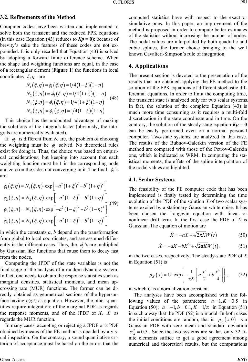 C. FLORIS 981 3.2. Refinements of the Method Computer codes have been written and implemented to solve both the transient and the reduced FPK equations (in this case Equation (43) reduces to Kp = 0): because of brevity’s sake the features of these codes are not ex- pounded. It is only recalled that Equation (43) is solved by adopting a forward finite difference scheme. When the shape and weighting functions are equal, in the case of a rectangular element (Figure 1) the functions in local coordinates , are 11 22 33 44 ,,1411 ,), 1411 ,,1411 ,,1411 N N N N . (48) This choice has the undoubted advantage of making the solutions of the integrals faster (obviously, the inte- grals are numerically evaluated). If i is different from Ni are, the problem of choosing the weighting must be i solved. No theoretical rules exist for doing it. Thus, the choice was based on empiri- cal considerations, but keeping into account that each weighting function must be 1 in the corresponding node and zero on the sides not converging in it. The final i ’s are: ,(49) 22 22 11 22 22 22 22 22 33 22 22 44 ,,exp11 ,,exp11 ,,exp11 ,,exp11 Nab Nab Nab Nab in which the constants a, b depend on the transformation from global to local coordinates, and are assumed differ- ently in the different cases. Thus, the i ’s are multiplied by Gaussian like functions that cause them to decay fast from the nodes. Computing the JPDF of the state variables is not the final stage of the analysis of a random dynamic system. In fact, one needs to obtain the response statistics such as marginal densities, statistical moments, and mean up- crossing rate (MUR) functions. The former can be di- rectly obtained as geometrical sections of the hypersur- face having p(z,t) as equation. However, the other quan- tities require integration: of the marginal PDF as regards the response moments, and of the JPDF of X, as regards the MUR function. In many cases, accepting or rejecting a JPDF or a PDF obtained by means of the FE method is decided by a vis- ual inspection. On the contrary, a sound quantitative cri- terion of acceptance must be based on the errors that the computed statistics have with respect to the exact or simulative ones. In this paper, an improvement of the method is proposed in order to compute better estimates of the statistics without increasing the number of nodes. The nodal values are interpolated by both quadratic and cubic splines, the former choice bringing to the well known Cavalieri-Simpson’s rule of integration. 4. Applications The present section is devoted to the presentation of the results that are obtained applying the FE method to the solution of the FPK equations of different stochastic dif- ferential equations. In order to limit the computing time, the transient state is analyzed only for two scalar systems. In fact, the solution of the complete Equation (43) is much more time consuming as it requires a multi-fold discretization in the state coordinate and in time. On the contrary, the solution of the steady-state equation Kp = 0 can be easily performed even on a normal personal computer. Two-state systems are analyzed in this case. The results of the Bubnov-Galerkin version of the FE method are compared with those of the Petrov-Galerkin one, which is indicated as WRM. In computing the sta- istical moments, the effets of the spline interpolation of the nodal values are highlited. 4.1. Scalar Systems The feasibility of the FE computer code that has been implemented is firstly tested by determining the time evolution of the PDF of the solution X of two scalar sys- tems excited by a stationary Gaussian white noise. It has been chosen the Langevin equation with linear or nonlinear drift term. In the first case the PDF of X is Gaussian. The equation of motion are 2π aXKW t (50) 32π aXbXKW t . (51) in the two cases, respectively. The steady-state PDF of X in Equation (51) is 24 1 exp π24 Xxx px Cab K , (52) in which C is a normalization constant. The analyses have been accomplished with the fol- lowing values of the parameters: in Equation (50); 1, 0.5aK 1,0.1,1 πab K in Equation (51) in such a way that the PDF (52) is bimodal. In both cases the initial conditions are random, that is ,0 X px is a Gaussian PDF with zero mean and standard deviation . Since the two systems are scalar, only 32 fi- nite elements suffice to get a good agreement among numerical and theoretical results, but the computations 20.5 X Open Access ENG  C. FLORIS 982 are repeated every 0.01 s, that is t 0.01. The time evolutions of , X pxt are in Figures 2 and 3 for Equations (50) and (51), respectively. It is not sur- prising that the PDF of X depicted in Figure 2 converges very fast to the steady-state one as this is Gaussian like the initial one. However, the convergence is fast as in the case of the nonlinear Langevin equation even if the initial and the final PDF are quite different. p x t = 0 s p x t = 0.5 s p x t = 3.0 s Figure 2. Time evolution of the PDF p(x) of X in Equation (50), random initial condition: stars FE solution, line stea- dy-state Gaussian PDF. Figure 3. Time evolution of the PDF p(x) of X in Equation (51), random initial condition: stars FE solution, line stea- dy-state exact PDF. 4.2. Duffing Oscillator The second case that has been examined regards a Duff- ing oscillator excited by a Gaussian white noise. The go- verning equation of motion is 23 00 0 2 2π tXtXtX KW t t (53) where and are constant parameters, and W(t) is a unit strength Gaussian white noise. In this case, the steady- state JPDF is known to be [5] 242 2 0 ,exp π242 xxx pxx CK , (54) in which 00 2 , and C is a normalization constant, whose expression is 11 22 0140 πexp 88 K CK , (55) where 23 000 π2K and 14 K is the modified Bessel function of order 1/4. It is recalled that, when both and are positive, the PDF of X is unimodal and Gaussian like, while for the PDF is bimodal. An analytical solution is known also for the MUR function: 1 2 00 0 1 2 140 4 2 2 0 πexp 8 8 1 exp 42 XxK x x . (56) The computations have been performed for 00.10 rads , 00.20 , = 1 or 1, = 0.1, K = 0.4/; 600 elements have been used for 1, while 400 or 900 for = +1. The statistics of X are illustrated in Figures 4 and 5 for = 1 and 1, respectively. In both cases, the agreement is good with the exception of the MUR function of the case = 1, which shows a dis- crepancy near the peak. A visual inspection is not able to discriminate among the different approaches and degrees of approximation. Thus, the response statistical moments are to be considered. The response statistics are listed in Tables 1 and 2 for = 1 and 1, respectively. The errors are very limited as regards the statistical moments of both X and . The largest value of the MUR function X has a larger error, which is more pronounced in the case = 1. Us- ing weighting functions different from the shape func- tions (WRM) yields good results; in the case = 1 it re- quires a smaller number of elements, 400 against 900. The constants a, b in Equation (49) are taken equal to half the lengths of the element sides. The values of the PDF in the tails have been con- Open Access ENG  C. FLORIS 983 trolled. As regards pX(x), it is worth 6.194E04, 2.354E 07, 2.577E13 for x = 3.0 3.3 X , 4.0 4.4 X , 5.0 5.5 X , respectively, for = 1. The FE method yields 1.929E04, 7.596E08, and 2.635E14 in the three cases, respectively. Even if the errors are notable, on the other hand they are smaller than those caused by the equivalent linearization method. The estimates ob- tained for = 1 are analogous. x x pX x X Figure 4. Steady-state statistics of X for Duffing oscillator with = 1: top rendering of the two-dimensional JPDF of X , ; middle marginal PDF of X; bottom MUR function Xx . 4.3. Oscillator with Parametric Excitation Now, consider the dynamic system , (57) 2 00 2 01 2 21 1 XtXtXt Wt XtFXWt in which W1(t) and W2(t) are Gaussian uncorrelated white noises with power spectral densities K1 and K2, respec x x pX x X x Figure 5. Steady-state statistics of X for Duffing oscillator with = 1: top rendering of the two-dimensional JPDF of X ,; middle marginal PDF of X; bottom MUR function Xx (rhombs exact values, stars FE solution). Open Access ENG  C. FLORIS 984 tively. The oscillator of Equation (57), which has the parametric excitation W1(t), belongs to the class of gen- eralized stationary potential [14] if the condition 4 012 K is fulfilled. The steady-state JPDF has the form (27) with 222 00 00 1 21 , π2 xd xxxf K uu . (58) It is notable that , x does not depend on the in- Table 1. Response moments for X of Equation (53), = 1. (1) (2) (3) (4) 2 EX 400 0.806231 0.806231 0.817561 900 0.812513 0.812513 400* 0.813330 0.813330 4 EX 400 1.760082 1.759952 1.824386 900 1.795570 1.795544 400* 1.790557 1.790427 2 X 400 0.985652 0.985652 1.000 900 0.996163 0.996163 400* 0.995807 0.995807 4 EX 400 2.882954 2.882833 3.000 900 2.947204 2.947183 400* 3.015625 2.942821 max X(x) 400 0.168447 0.168433 0.168507 900 0.168476 0.168473 400* 0.168517 - (1) number of elements. (2) Quadratic spline. (3) Cubic spline. (4) Exact value. * WRM. Table 2. Response moments of X in Equation (53), = 1. (1) (2) (3) 2 X 8.685545 8.68555 8.713629 8.67606* 8.67607* 4 EX 96.3825 96.38228 97.13629 96.3920* 96.39178* 2 EX 0.996163 0.996163 1.000 1.00645* 1.00645* 4 X 2.947204 2.94282 3.000 3.01563* 3.01551* max X(x) 0.101775 0.101767 0.118085 0.101702* - (1) Quadratic spline. (2) Cubic spline. (3) Exact value. *WRM. Results obtained with 600 elements. tensity of the parametric excitation W1(t). The computations have been performed for the fol- lowing set of parameters: 23 11cm sK, 23 210 cmsK, 02πrads, 00.02, 2 010sin 2π X X. In the Bubnov-Galerkin approach, meshes with 400 and 900 elements have been tested. In the Petrov-Galerkin approach, the elements over one quarter of the integration domain are 400, and the constants a, b of Equation (49) are both 0.150. The exact stationary PDF of X and those obtained by using the FE method are compared in the top plot of Figure 6. Again, both methods and all levels of discreti- zation give good results so that they cannot be discrimi- nated by a visual inspection. It is not possible to distin- guish the PDF of the Bubnov-Galerkin approach from that obtained with different weighting and shape func- tions. The bottom plot compares the MUR functions X . In this case, an analytical expression does not exist: the results labeled as exact are obtained inserting the exact JPDF in the Rice’s formula, then the integral is numerical evaluated. The same procedure is used to ob- tain X from the FE results. The agreement is quite satisfactory. The mean square values of X and are in Table 3. pX x X x Figure 6. Steady-state statistics of X in Equation (57): top marginal PDF of X; bottom MUR function Xx (stars exact values, circles, crosses and triangles FE solutions). Open Access ENG  C. FLORIS 985 Table 3. Response moments of X in Equation (57). (1) (2) (3) 2 EX 3.123129 3.123132 3.252787 3.128027* 3.127946* 2 EX 124.3301 124.3301 124.9997 125.2834* 125.2834* max X(x) 1.0244 - 1.0199 1.0244* - (1) Simpson's rule of integration. (2) Cubic spline. (3) Exact value. *WRM. There are reported only the values obtained by means of 900 elements in the Bubnov’s approach and 400 in the Petrov’s one. It is evident that the errors are small in any case. However, Petrov’s procedure allows a non negligi- ble computing time saving. 4.4. Oscillator with Cubic Damping and Stiffness Consider the following oscillator 32 3 0 tXtXtXtX t , (59) where 00 2, 1, 1 , and , are nonlinear parameters. The FPK equation associated with this oscil- lator does not admit an analytical solution. Thus, the fi- nite element estimates have been compared with those obtained by means of Monte Carlo simulation. Sets with 60,000 samples of motion histories have been simulated. The parameters take the following values: 02π, 0.02, 1. Because of space limitations only the marginal PDF’s of X for = 1 are shown in Figure 7, and only for 800 elements over one quarter of the domain with shape functions different from weighting functions. A perfect agreement between the two curves can be noted. This is confirmed by the statistical moments: by simula- tion, and by means of the FE method. However, the former re- quires more than 9 hours of elaboration on a workstation with quadcore processor, while the latter few minutes. 20.102583,EX 2 EX 40.0252177EX 0.101999, 40.02EX 49447 5. Conclusions This paper aims at giving a contribution to some ques- tions regarding the FE method for solving the FPK equa- tio n, which remains unanswered or partially answered. Firstly, the existence domain of a JPDF p(z,t) is generally infinite, while the FE solution is restricted to a limited domain. This fact has two shortcomings: 1) the former is the necessity of having a good estimate of the response standard deviations in order to give the integration do- Figure 7. Steady-state PDF of X in Equation (59): blue line WRM FE estimate, black line monte carlo simulation). main appropriate dimensions; 2) no precise information is obtained on the values of the JPDF in its tails, which are very important in structural reliability. An enlarge- ment of the domain of integration causes a notable in- crease of the computations in many cases. According to Langley [47], a combination of finite elements with boundary elements or infinite elements does not seem to be effective in the case of the FPK equation. A second question is in some way related to the former: spurious oscillations of the PDF values and meaningless regions of negative values are possible, particularly in the tails, when the mesh is too coarse or badly defined. Fi- nally, the application of the FE method to problems with more than 3 dimensions is an open question because of computer storage and speed requirements. Computer programs have been written and imple- mented for both formulations of the FE method: the Bubnov-Galerkin method, which uses equal weighting and shape functions, and the Petrov-Galerkin method in which these functions are different. Examining the results that have obtained for different stochastic systems with additive or both additive and multiplicative excitations, the following conclusions can be drawn: 1) The FE method is very feasible for solving the reduced FPK equation when the response states are few, say not more than three or four. If there are more states, programming is more cumbersome, and the com- puting times are unavoidably longer, not competitive with Monte Carlo simulation. 2) The steady-state statis- tical moments of the response are computed with small errors and a reasonable charge for computations. For two states, this is lesser than that required by a Monte Carlo simulation, and larger than that required by a moment equation approach. The FE method has the advantage that no closure schemes are required for computing the moments differently from the moment equation approach. 3) If one wants to limit the charge for computations, the Open Access ENG  C. FLORIS 986 integration domain must be kept into 4 - 5 standard deviations of the variables. In this way, it is not possible to get reliable values in the tails of the JPDF, in which negative values can be encountered. 4) The use of weighting functions different from shape functions has given encouraging results so that further study in this direction seems to be promising. 5) The FE method is proved to be feasible even for transient responses, but in this case the computing time increases dramatically as the equations are to be solved in every time instant. REFERENCES [1] A. T. Bharucha-Reid, “Elements of Theory of Markov Processes and Their Applications,” McGraw Hill, New York, 1960. [2] R. L. Stratonovich, “Topics in the Theory of Random Noise,” Gordon and Breach, New York, 1963. [3] Y. K. Lin and G. Q. Cai, “Probabilistic Structural Dyna- mics: Advanced Theory and Applications,” McGraw Hill, New York, 1995. [4] H. Risken, “Fokker-Planck Equation: Methods of Solu- tion and Applications,” Springer, Berlin, 1996. [5] T. K. Caughey, S. H. Crandall and R. H. Lyon, “Deriva- tion and Application of the Fokker-Planck Equation to Discrete Nonlinear Dynamic Systems,” Journal of Acous- tical Society of America, Vol. 35, No. 11, 1963, pp. 1683- 1692. http://dx.doi.org/10.1121/1.1918788 [6] T. K. Caughey and H. J. Payne, “On the Response of a Class of Self-Excited Oscillators to Stochastic Excita- tion,” International Journal of Non-Linear Mechanics, Vol. 2, No. 2, 1967, pp. 125-151. http://dx.doi.org/10.1016/0020-7462(67)90010-8 [7] A. T. Fuller, “Analysis of Nonlinear Stochastic Systems by Means of the Fokker-Planck Equation,” International Journal of Control, Vol. 9, No. 6, 1969, pp. 603-655. http://dx.doi.org/10.1080/00207176908905786 [8] S. C. Liu, “Solutions of Fokker-Planck Equation with Ap- plications in Nonlinear Random Vibration,” Bell System Technical Journal, Vol. 48, No. 8, 1969, pp. 2031-2051. http://dx.doi.org/10.1002/j.1538-7305.1969.tb01163.x [9] M. F. Dimentberg, “An Exact Solution to a Certain Non- Linear Random Vibration Problem,” International Jour- nal of Non-Linear Mechanics, Vol. 17, No. 4, 1982, pp. 231-236. http://dx.doi.org/10.1016/0020-7462(82)90023-3 [10] T. K. Caughey and F. Ma, “The Steady-State Response of a Class of Dynamical Systems to Stochastic Excitation,” Journal of Applied Mechanics ASME, Vol. 49, No. 3, 1982, pp. 629-632. http://dx.doi.org/10.1115/1.3162538 [11] T. K. Caughey and F. Ma, “The Exact Steady-State Solu- tion of a Class of Non-Linear Stochastic Systems,” In- ternational Journal of Non-Linear Mechanics, Vol. 17, No. 3, 1982, pp. 137-142. http://dx.doi.org/10.1016/0020-7462(82)90013-0 [12] T. K. Caughey, “On the Response of Non-Linear Oscilla- tors to stochastic Excitation,” Probabilistic Engineering Mechanics, Vol. 1, No. 1, 1986, pp. 2-4. http://dx.doi.org/10.1016/0266-8920(86)90003-2 [13] Y. Yong and Y. K. Lin, “Exact Stationary Response So- lution for Second Order Nonlinear Systems under Para- metric and External White Noise Excitations,” Journal of Applied Mechanics ASME, Vol. 54, No. 2, 1987, pp. 414- 418. http://dx.doi.org/10.1115/1.3173029 [14] Y. K. Lin and G. Q. Cai, “Exact Stationary Response Solution for Second Order Nonlinear Systems under Pa- rametric and External White Noise Excitations: Part II,” Journal of Applied Mechanics ASME, Vol. 55, No. 3, 1988, pp. 702-705. http://dx.doi.org/10.1115/1.3125852 [15] G. Q. Cai and Y. K. Lin, “On Exact Stationary Solutions of Equivalent Non-Linear Stochastic Systems,” Interna- tional Journal of Non-Linear Mechanics, Vol. 23, No. 4, 1988, pp. 315-325. http://dx.doi.org/10.1016/0020-7462(88)90028-5 [16] C. Soize, “Steady-State Solution of Fokker-Planck Equa- tion in Higher Dimension,” Probabilistic Engineering Mechanics, Vol. 3, No. 4, 1988, pp. 196-206. http://dx.doi.org/10.1016/0266-8920(88)90012-4 [17] W.-Q. Zhu, G. Q. Cai and Y. K. Lin, “On Exact Station- ary Solutions of Stochastically Perturbed Hamiltonian Systems,” Probabilistic Engineering Mechanics, Vol. 5, No. 2, 1990, pp. 84-87. http://dx.doi.org/10.1016/0266-8920(90)90011-8 [18] W.-Q. Zhu, “Exact Solutions for Stationary Responses of Several Classes of Nonlinear Systems to Parametric and/ or External White Noise Excitations,” Applied Mathe- matics and Mechanics, Vol. 11, No. 2, 1990, pp. 165-175. http://dx.doi.org/10.1007/BF02014541 [19] C. Soize, “Exact Stationary Response of Multi-Dimen- sional Non-Linear Hamiltonian Dynamical Systems under Parametric and External Stochastic Excitations,” Journal of Sound and Vibration, Vol. 149, No. 1, 1991, pp. 1-24. http://dx.doi.org/10.1016/0022-460X(91)90908-3 [20] W.-Q. Zhu and Y. Q. Yang, “Exact Stationary Solutions of Stochastically Excited and Dissipated Integrable Ham- iltonian Systems,” Journal of Applied Mechanics ASME, Vol. 63, No. 2, 1996, pp. 493-500. http://dx.doi.org/10.1115/1.2788895 [21] R. Wang and K. Yasuda, “Exact Stationary Probability Density for Second Order Nonlinear Systems under Ex- ternal White Noise Excitation,” Journal of Sound and Vi- bration, Vol. 205, No. 5, 1997, pp. 647-665. http://dx.doi.org/10.1006/jsvi.1997.1052 [22] R. Wang and Z. Zhang, “Exact Stationary Response So- lutions of Six Classes of Nonlinear Stochastic Systems under Stochastic Parametric and External Excitations,” Jou r na l o f E n gi ne e ring Mechanics ASCE, Vol. 124, No. 1, 1998, pp. 18-23. http://dx.doi.org/10.1061/(ASCE)0733-9399(1998)124:1( 18) [23] Z. Zhang, R. Wang and K. Yasuda, “On Joint Stationary Probability Density Function of Nonlinear Dynamic Sys- tems,” Acta Mechanica, Vol. 130, No. 1, 1998, pp. 29-39. http://dx.doi.org/10.1007/BF01187041 [24] R. Wang, K. Yasuda and Z. Zhang, “A Generalized Ana- lysis Technique of the Stationary FPK Equation in Non- Open Access ENG  C. FLORIS 987 linear Systems under Gaussian White Noise Excitations,” International Journal of Engineering Science, Vol. 38, No. 12, 2000, pp. 1315-1330. http://dx.doi.org/10.1016/S0020-7225(99)00081-6 [25] R. Wang and Z. Zhang, “Exact Stationary Solutions of the Fokker-Planck Equation for Nonlinear Oscillators under Stochastic Parametric and External Exctations,” Nonlinearity, Vol. 13, No. 3, 2000, pp. 907-920. [26] Z. L. Huang and W.-Q. Zhu, “Exact Stationary Solutions of Stochastically and Harmonically Excited and Dissipat- ed Integrable Hamiltonian Systems,” Journal of Sound and Vibration, Vol. 230, No. 3, 2000, pp. 709-720. http://dx.doi.org/10.1006/jsvi.1999.2634 [27] W.-Q. Zhu and Z. L. Huang, “Exact Stationary Solutions of Stochastically Excited and Dissipated Integrable Ham- iltonian Systems,” International Journal of Non-Linear Mechanics, Vol. 36, No. 1, 2001, pp. 3-48. http://dx.doi.org/10.1016/S0020-7462(99)00086-4 [28] R. G. Bhandari and R. E. Sherrer, “Random Vibration in Discrete Nonlinear Dynamic Systems,” Journal of Me- chanical Engineering Science, Vol. 10, No. 2, 1968, pp. 168-174. http://dx.doi.org/10.1243/JMES_JOUR_1968_010_024_0 2 [29] G. Muscolino, G. Ricciardi and M. Vasta, “Stationary and Non-Stationary Probability Density Function for Non- Linear Oscillators,” International Journal of Non-Linear Mechanics, Vol. 32, No. 6, 1997, pp. 1051-1064. http://dx.doi.org/10.1016/S0020-7462(96)00134-5 [30] G.-K. Er, “Multi-Gaussian Closure Method for Randomly Excited Non-Linear Systems,” International Journal of Non-Line ar Mechanics, Vol. 33, No. 2, 1998, pp. 201-214. http://dx.doi.org/10.1016/S0020-7462(97)00018-8 [31] G.-K. Er, “A Consistent Method for the Solution to Re- duced FPK Equation in Statistical Mechanics,” Physica A, Vol. 262, No. 1-2, 1999, pp. 118-128. http://dx.doi.org/10.1016/S0378-4371(98)00362-8 [32] M. Di Paola and A. Sofi, “Approximate Solution of the Fokker-Planck-Kolmogorov Equation,” Probabilistic En- gineering Mechanics, Vol. 17, No. 4, 2002, pp. 369-384. http://dx.doi.org/10.1016/S0266-8920(02)00034-6 [33] W. Martens, U. von Wagner and V. Mehrmann, “Calcula- tion of High-Dimensional Probability Density Functions of Stochastically Excited Nonlinear Mechanical Sys- tems,” Nonlinear Dynamics, Vol. 67, No. 3, 2012, pp. 2089-2099. http://dx.doi.org/10.1007/s11071-011-0131-2 [34] J. D. Atkinson, “Eigenfunction Expansions for Randomly Excited Non-Linear Systems,” Journal of Sound and Vi- bration, Vol. 30, No. 2, 1973, pp. 153-172. http://dx.doi.org/10.1016/S0022-460X(73)80110-5 [35] Y.-K. Wen, “Approximate Method for Nonlinear Random Vibration,” Journal of Engineering Mechanics Division ASCE, Vol. 101, No. 4, 1975, pp. 389-401. [36] J. P. Johnson and R. A. Scott, “Extension of Eigenfunc- tion Expansion of a Fokker-Planck Equation—I. First Order System,” International Journal of Non-Linear Me- chanics, Vol. 14, No. 5-6, 1979, pp. 315-324. http://dx.doi.org/10.1016/0020-7462(79)90005-2 [37] J. P. Johnson and R. A. Scott, “Extension of Eigenfunc- tion Expansion of a Fokker-Planck Equation—II. Second Order System,” International Journal of Non-Linear Me- chanics, Vol. 15, No. 1, 1980, pp. 41-56. http://dx.doi.org/10.1016/0020-7462(80)90052-9 [38] U. von Wagner and W. V. Wedig, “On the Calculation of Stationary Solutions of Multi-Dimensional Fokker-Planck Equations by Orthogonal Functions,” Nonlinear Dynamic s, Vol. 21, No. 3, 2000, pp. 289-306. http://dx.doi.org/10.1023/A:1008389909132 [39] R. Courant and D. Hilbert, “Methods of Mathematical Physics,” John Wiley & Sons, New York, 1989. [40] J. B. Roberts, “First-Passage Time for Randomly Excited Non-Linear Oscillators,” Journal of Sound and Vibration, Vol. 109, No. 1, 1986, pp. 33-50. http://dx.doi.org/10.1016/S0022-460X(86)80020-7 [41] T. Blum and A. J. McKane, “Variational Schemes in the Fokker-Planck Equation,” Journal of Physics A: Mathe- matical and General, Vol. 29, No. 9, 1996, pp. 1859- 1872. http://dx.doi.org/10.1088/0305-4470/29/9/003 [42] M. Dehghan and M. Tatari, “The Use of He’s Variational Iteration Method for Solving a Fokker-Planck Equation”, Physica Scripta, Vol. 74, No. 3, 2006, pp. 310-316. http://dx.doi.org/10.1088/0031-8949/74/3/003 [43] A. Quarteroni and A. Valli, “Numerical Approximation of Partial Differential Equations,” Springer, Berlin, 1994. [44] L. A. Bergman and J. C. Heinrich, “Solution of the Pon- triagin-Vitt Equation for the Moments of Time to First Passage of the Randomly Accelerated Particle by the Fi- nite Element Method,” International Journal for Nu- merical Methods in Engineering, Vol. 15, No. 9, 1980, pp. 1408-1412. http://dx.doi.org/10.1002/nme.1620150913 [45] L. A. Bergman and J. C. Heinrich, “On the Moments of Time to First Passage of Linear Oscillator,” Earthquake Engineering and Structural Dynamics, Vol. 9, No. 3, 1981, pp. 197-204. http://dx.doi.org/10.1002/eqe.4290090302 [46] B. F. Spencer Jr. and L. A. Bergman, “On the Reliability of a Simple Hysteretic System,” Journal of Engineering Mechanics, Vol. 111, No. 12, 1985, pp. 1502-1514. http://dx.doi.org/10.1061/(ASCE)0733-9399(1985)111:12 (1502) [47] R. S. Langley, “A Finite Element Method for the Statis- tics of Non-Linear Random Vibration,” Journal of Sound and Vibration, Vol. 101, No. 1, 1985, pp. 41-54. http://dx.doi.org/10.1016/S0022-460X(85)80037-7 [48] H. P. Langtangen, “A General Numerical Solution Method for Fokker-Planck Equations with Applications to Structural Reliability,” Probabilistic Engineering Mechanics, Vol. 6, No. 1, 1991, pp. 33-48. http://dx.doi.org/10.1016/S0266-8920(05)80005-0 [49] B. F. Spencer Jr. and L. A. Bergman, “On the Numerical Solution of the Fokker-Planck Equation for Nonlinear Sto- chastic Systems,” Nonlinear Dynamics, Vol. 4, No. 4, 1993, pp. 357-372. http://dx.doi.org/10.1007/BF00120671 [50] H. U. Köylüoglu, S. R. K. Nielsen and R. Iwankiewicz, “Reliability of Non-Linear Oscillators Subject to Poisson Open Access ENG  C. FLORIS Open Access ENG 988 Driven Impulses,” Journal of Sound and Vibration, Vol. 176, No. 1, 1994, pp. 19-33. http://dx.doi.org/10.1006/jsvi.1994.1356 [51] L.-C. Shiau and T.-Y. Wu, “A Finite Element Method for Analysis of Non-Linear System under Stochastic Para- Metric and External Excitation,” International Journal of Non-Linear Mechanics, Vol. 31, No. 2, 1996, pp. 193- 201. http://dx.doi.org/10.1016/0020-7462(95)00049-6 [52] L. A. Bergman, S. F. Wojtkiewicz, E. A. Johnson and B. F. Spencer Jr., “Robust Numerical Solution of the Fok- ker-Planck Equation for Second Order Dynamical Sys- tems under Parametric and External White Noise Excita- tion,” In: W. H. Kliemann, Ed., Nonlinear Dynamics and Stochastic Mechanics, American Mathematical Society, Providence, 1996, pp. 23-37. [53] A. Masud and L. A. Bergman, “Application of Multi-Scale Finite Element Methods to the Solution of the Fokker- Planck Equation,” Computer Methods in Applied Mechan- ics and Engineering , Vol. 194, No. 12-16, 2005, pp. 1513- 1526. http://dx.doi.org/10.1016/j.cma.2004.06.041 [54] M. Kumar, S. Chakravorty, P. Singla and J. L. Junkins, “The partition of Unity Finite Element Approach with Hp-Refinement for the Stationary Fokker-Planck Equa- tion,” Journal of Sound and Vibration, Vol. 327, No. 1-2, 2009, pp. 144-162. http://dx.doi.org/10.1016/j.jsv.2009.05.033 [55] E. Wong and M. Zakai, “On the Relation between Ordinary and Stochastic Equations,” International Journal of Engi- neering Science, Vol. 3, No. 2, 1965, pp. 213-229. http://dx.doi.org/10.1016/0020-7225(65)90045-5 [56] R. L. Stratonovich, “Topics in Theory of Random Noise,” Taylor & Francis, New York, 1967. [57] K. Itô, “On Stochastic Differential Equations,” Memoirs of American Mathematical Society, Vol. 4, 1951, pp. 1-51. [58] K. Itô, “On a Formula Concerning Stochastic Differen- tials,” Nagoya Mathematical Journal, Vol. 3, No. 1, 1951, pp. 55-65. [59] M. Di Paola, “Stochastic Differential Calculus,” In: F. Casciati, Ed., Dynamic Motion: Chaotic and Stochastic Behaviour, Springer Verlag, Wien, 1993, pp. 29-92. [60] W. Q. Zhu, “Nonlinear Stochastic Dynamics and Control in Hamiltonian Formulation,” Applied Mechanics Review, Vol. 59, No. 4, 2006, pp. 230-248. http://dx.doi.org/10.1115/1.2193137 [61] J. B. Roberts and P. Spanos, “Random Vibration and Statistical Linearization,” John Wiley & Sons, New York, 1990.
|