Journal of Water Resource and Protection
Vol.08 No.01(2016), Article ID:62712,15 pages
10.4236/jwarp.2016.81004
Assessment of Climate Change for Precipitation and Temperature Using Statistical Downscaling Methods in Upper Godavari River Basin, India
Vidya R. Saraf1,2, Dattatray G. Regulwar1
1Department of Civil Engineering, Government College of Engineering, Jalgaon, Maharashtra State, India
2Department of Civil Engineering, Government College of Engineering, Aurangabad, Maharashtra State, India

Copyright © 2016 by authors and Scientific Research Publishing Inc.
This work is licensed under the Creative Commons Attribution International License (CC BY).
http://creativecommons.org/licenses/by/4.0/


Received 25 November 2015; accepted 10 January 2016; published 13 January 2016
ABSTRACT
In the present study SDSM downscaling model was used as a tool for downscaling weather data statistically in upper Godavari river basin. Two Global Climate Models (GCMs), CGCM3 and HadCM3, have been used to project future maximum temperature (Tmax), minimum temperature (Tmin) and precipitation. The predictor variables are extracted from: 1) the National Centre for Environmental Prediction (NCEP) reanalysis dataset for the period 1961-2003, 2) the simulations from the third-generation Hadlycentre Coupled Climate Model (HadCM3) and Coupled Global Climate Model (CGCM3) variability and changes in Tmax, Tmin and precipitation under scenarios A1B and A2 of CGCM3 model and A2 and B2 of HadCM3 model have been presented for future periods: 2020s, 2050s and 2080s. The scatter-plots and cross-correlations are used for verifying the reliability of the simulation. Maximum temperature increases in future for almost all the scenarios for both GCMs. Also downscaled future precipitation shows increasing trends for all scenarios.
Keywords:
Downscaling, CGCM3, HadCM3, Scenario, Temperature, Precipitation

1. Introduction
The change in frequency, timing, and amount of precipitation will affect river flow and occurrence of floods and droughts. The third assessment report of the Intergovernmental Panel on Climate Change [1] reported the general impact of climate change on water resources and indicated an intensification of the global hydrological cycle affecting both ground and surface water supplies. GCMs are the most advanced tools that are available for the simulation of future climate [2] . These models are capable of predicting climate, hundreds of years into future considering the GHG concentrations in the atmosphere. GCMs as the most credible tools designed to simulate time series of climate variables, considering the concentrations of GHGs [3] . However, understanding the influence of climate change on the hydrological cycle on a global scale is inadequate for water resource planners at basin level due to their coarse (grid) resolution and the local heterogeneity of terrain and climate [1] [4] . A significant amount of effort has been expended in assessing the potential impact of climate change on basin water resources [5] -[8] .
Wilby et al. [9] have studied downscaling techniques and stated that using downscaling techniques, GCM outputs can be changed into surface variables in the scale of the basin under study. Tisseuil et al. [10] have stated that downscaling bridges the large scale atmospheric conditions with local scale climatic data. There are different methods for creating local climate scenarios from GCM climate scenarios. Downscaling techniques are broadly classified into two categories as dynamic downscaling and statistical downscaling. In dynamic downscaling a Regional Climatic Model (RCM) is nested in a GCM. The RCM is an atmospheric physics based model to which boundary conditions are provided with the output of a GCM. The major drawback of dynamic downscaling is its complexity and high computation cost [2] . The other problem with dynamic downscaling is the propagation of systematic bias from GCM to RCM [11] . Statistical downscaling methods construct statistical relationships between the large scale GCM outputs (predictors) and the catchment scale climate variables (predictands). The basic advantage of statistical downscaling is that it is computationally less demanding compared to dynamic downscaling.
According to Wilby and Wigly [12] , statistical downscaling is based on few assumptions. These assumptions are that the predictor-predictand relationships are valid under future climatic conditions, and predictor variables and their changes are well characterized by GCMs. In general, statistical downscaling techniques are classified into three main categories as weather classification, regression models and weather generators. Weather classification methods classify large scale atmospheric variables of GCMs into finite number of states and relate them to basin scale climate variables. Regression methods build up linear or nonlinear functions between predictors and predictands. Weather generators produce a synthetic series of climate data, while preserving statistical attributes of the observations of climate variables [13] .
In downscaling there are various sources of uncertainty like GCM uncertainty, which is due to incomplete knowledge about the underlying geophysical processes of global change, coarse grid resolutions and unresolved processes lead to limitations in the accuracy of the models. Scenario uncertainty results from unpredictability in the forecast of future socioeconomic and human behavior resulting in future greenhouse gas (GHG) emission scenarios. Downscaled outputs of a single GCM with a single climate change scenario represent a single trajectory among a number of realizations derived using various scenarios with GCMs. Such a single trajectory alone cannot represent a future hydrologic scenario, and will not be useful in assessing hydrologic impacts due to climate change [3] .
There are three objectives of this study. The first objective is to investigate the adaptability of SDSM in downscaling precipitation and temperature for basins. The second objective is to produce average monthly local- scale precipitation time series reflective of climate change signals obtained by downscaling from GCM predictors. The third objective is to find out the dry and wet spell length. To overcome the single GCM and single scenario uncertainty two GCM (CGCM3 and Had CM3) and A1B, A2 and B2 scenarios have been used. This study provides a valuable dataset for climate change impact applications with regard to water resources in study region.
2. Catchment Description
Godavari rises in the Sahyadri hills near Triambakeswar, about 80 km from the shore of Arabian Sea, at an elevation of 1067 m in the Nasik district of Maharashtra state, India. After flowing for about 1465 km in a general south-easterly direction through Maharashtra and Andhra Pradesh, Godavari falls into the Bay of Bengal north of Rajahmundry. The basin lies between latitudes 16˚16'0"N and 23˚43'N longitudes 73˚26'E and 83˚07'E. The basin extends over an area of 312,813 km2, which is nearly 10% of the total geographical area of the country. It is bounded on the north by the Satmala Hills, the Ajanta Range and the Mahadeo Hills, on the east and south by the Eastern Ghats and on the west by the Western Ghats. The study area of the research is the upper Godavari basin in Maharashtra state in India. The mean monthly Tmax in the upper Godavari basin varies from 29.64 to 38.60 and mean annual Tmax is 32.45. The mean monthly Tmin ranges from 14.38 to 25.12 based on decadal (1961-2007) observed values (Figure 1).
3. Data Extraction
1) Reanalysis data
The monthly mean atmospheric variables were derived from the National Centre for Environmental Prediction (NCEP/NCAR) reanalysis dataset for the period from January 1961 to December 2003. The data have a horizontal resolution of 2.5˚ × 2.5˚ and seventeen constant pressure levels in the vertical.
2) GCM data
The GCMs selected in this study are CGCM3 (3.75˚ latitude × 3.75˚ longitude) and HadCM3 (2.5˚ latitude × 3.75˚ longitude). CGCM3 is developed by Canadian Centre for Climate Modelling and Analysis, whereas HadCM3 by Hadley Centre for Climate Prediction and Research/Met Office, UK, respectively. The future scenarios considered in this study are A1B and A2 for CGCM3 model and A2 and B2 for HadCM3 model, respectively. The predictor variables are available for period 1961-2100 for CGCM3 model, 1961-2099 for HadCM3 model. The selection of CGCM3 and HadCM3 is made on the basis of literature review and availability of data in SDSM compatible format. Further, these two models have been extensively used in statistical downscaling of climate variables over Indian Sub-continent [2] [19] [20] . The gridded predictor variables of NCEP/NCAR, CGCM3 and HadCM3 for the nearest grid in study area have been directly downloaded from the websites of Data Access Integration (DAI) (http://loki.qc.ec.gc.ca/DAI/predictors-e.html) and Canadian Climate Impacts Scenarios (CCIS) (http://www.cics.uvic.ca/scenarios/index.cgi) respectively. The predictors are simulated under
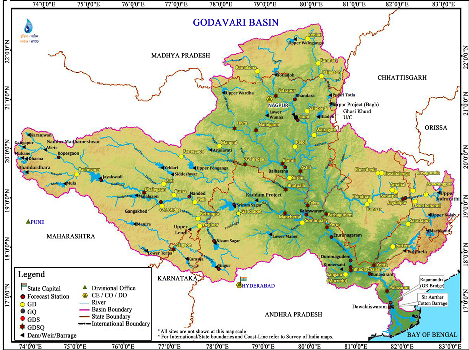
Figure 1. Basin map of Godavari basin.
historical GHG and aerosol concentration experiment (20C3M) as well as Special Report on Emission Scenarios (SRES) A2 for future run for CGCM3 model and HadCM3 model respectively.
3) Observed data obtained from Indian Metrological Department (IMD), Pune India in gridded format has been used in this study.
4. Methodology
Statistical Down-Scaling Model (SDSM) was developed by Wilby and Dawson [9] has been used to construct climate change scenarios for the catchment of Upper Godavari in Maharashtra. SDSM as a statistical tool was adopted due to several advantages such as low cost and user friendly over dynamical methods. There are many studies which have used SDMS in climate change impact assessments [14] -[16] . Regression method establishes a linear or nonlinear regression between predictands and predictors. Therefore, this method is highly depends on the empirical statistical relationships. The main advantage of it is simplicity and less computationally demanding of running the regression statistical method. However it is limited to the locations where good regression results could be found.
In SDSM, generation of station scale weather parameters is linearly conditioned by observed large scale predictors of atmosphere ( ). The downscaled process is either unconditional or conditional. The down- scaling for the conditional process like daily PCP depends on an intermediate variable such as occurrence of a wet day. The occurrence of wet day (
 ) on day i is linearly dependent on predictors
  (Equation (1))
 (1)
(1)
under the constraint . The value of
  varies according to prevailing large-scale weather conditions (represented by the predictor variables) between 0 and 1. The precipitation will occur if uniform random number
 .
.  is not a Boolean (0 or 1) number but is a continuous variable between 0 and 1. For example, on a day with high pressure,
  might be equal to 0.2. Then, r is used to determine whether a rainy day will actually occur depending upon whether r ≤ 0.2. The amount of total PCP (Pi) downscaled on day i with return of wet day is given by Equation (2)
 (2)
(2)
where k is a transformation (fourth root, inverse normal or logarithmic) which is applied, as PCP data is skewed in nature. In case of unconditional processes like daily temperature (Tmax and Tmin), a direct linear relationship is established between the predictand Ui and selected NCEP/NCAR predictors Xij on individual sites shown in Equation (3)
 (3)
(3)
where Ui is temperature on day i and  is selected NCEP/NCAR predictors on day i.
 ,
,  and
and  are regression coefficients estimated for each month using least-squares regression and
  is model error. It is generated stochastically using a series of serially independent Gaussian numbers and is added to the deterministic components on daily basis.
The various steps followed in the present study for downscaling and scenario generation are shown in Figure 2.
4.1. Quality Control Check, Transformation and Screening of Probable Predictors
Station-based meteorological data may have errors in terms of missing records or outliers. Quality control check function is used to identify such errors prior to model calibration. The missing data may be replaced by a data identifier code, i.e., −999. SDSM provides facility to transform data before calibration using different types of transformations such as logarithm, power, inverse, lag, binomial, etc. After quality control check and transformation, screen variable operation is applied to select appropriate sets of observed predictors from the suite of NCEP/NCAR reanalysis datasets based on scatter plots, correlation and partial correlation statistics [17] . Table 1 shows the predictors used in downscaling process.

Figure 2. Flow chart showing steps involved in downscaling and scenario generation (modified after Wilby and Dawson, 2007).

Table 1. NCEP predictors used in the screening process.
4.2. Calibration and Validation
SDSM is calibrated using observed station scale data (Tmax, Tmin and PCP) and screened sets of observed predictors, i.e., NCEP/NCAR reanalysis datasets. SDSM offers three different types of sub models; 1) monthly, 2) seasonal, and 3) annual for the downscaling of predictands (Tmax, Tmin and PCP) from the large scale predictors. The monthly sub model derives 12 different regression equations, one for each month, whereas seasonal sub model generates four different regression equations, one for each season. In case of annual sub model, a single regression equation is generated for all 12 months having same model parameters. The process involved in downscaling may be either unconditional (e.g., Tmax, Tmin) or conditional (e.g., PCP). There are two methods for optimizing SDSM; 1) Dual Simplex and 2) Ordinary Least Squares. Both the methods provide comparable results but Ordinary Least Squares is much faster and has been used in the present study. Further, monthly sub model type is preferred because there are large monthly variations in Tmax, Tmin and PCP at different stations within the study region. In monthly sub model, identical sets of predictors and predictands generate different statistical values for each month.
4.3. Generation of Present and Future Time Series for Tmax, Tmin and PCP
After calibrating the model, Weather Generator function is applied to generate ensembles of synthetic daily time series of Tmax, Tmin and PCP representing present climate from screened sets of NCEP/NCAR predictors. The synthetically generated daily time series of Tmax, Tmin and PCP is compared (in terms of statistics) with observed records to know how close it is to the present climate. Finally, Scenario Generator function is used to simulate future time series of Tmax, Tmin and PCP using outputs of GCMs (CGCM3 and HadCM3) on daily time-step under different emission scenarios.
5. Bias Correction
In this study, bias correction (BC), which is discussed in detail below, is also applied to the downscaled data obtained from the SDSMs using HadCM3 and CGCM predictors, in order to obtain a more realistic and unbiased data of future climate. The bias correction approach is used to eliminate the biases from the daily time series of downscaled data [18] -[20] . In this method, the biases are obtained by subtracting (in the case of temperature) the long-term monthly mean (1971-1990, 20 years) of observed data, from the mean monthly simulated control data (downscaled data by SDSM for the period of 1971-1990, 20 years), and dividing (in the case of precipitation) the long-term observed monthly mean data with simulated control data. The biases are then adjusted with the future downscaled daily time series according to their respective months. Equation (4) and Equation (5) are used to de-bias daily temperature and precipitation data.
 (4)
(4)
 (5)
(5)
where  and
and  are the de-biased (corrected) daily time series of temperature and precipitation respectively for future periods. SCEN represents the scenario data downscaled by SDSM for future periods (e.g., 2011-2099), and CONT represents downscaled data by SDSM for the present period (e.g., 1961-2000).
  and
and  are the daily time series of temperature and precipitation generated by SDSM for future periods respectively.
  and
and  are the long term mean monthly values for temperature and precipitation respectively for the control period simulated by SDSM.
  and
and  represent the long-term mean monthly observed values for temperature and precipitation. The bar on T and P shows the long-term average. The frequency and intensity of precipitation are the two main factors affecting precipitation variability [21] . The application of this method of study is to correct the precipitation amount and not the frequency, and also to remove any systematic errors belonging to SDSM during downscaling. It is assumed that the frequency is accurately simulated by SDSM.
6. Result and Discussion
In statistical downscaling, screening of suitable predictors for downscaling predictands is one of the most important steps. The explanatory power of individual predictor variable varies both spatially and temporally [9] . The choice of predictors can be different for different geographical regions depending on the properties of the predictor and the predictand to be downscaled [2] . On the basis of the correlation values and scatter plots, the selected suitable predictors for downscaling the temperatures and daily precipitation values for this case study are listed in Table 2.
The calibrate model takes up each of the predictand and a set of probable predictors and computes the parameters of multiple regression equations by using an optimization algorithm (ordinary least squares). Monthly model type is selected in which different model parameters are derived for each month. From the 20 years of data representing current climate (1961-1980) have been used for calibrating the regression model whereas 20 years of data (1981-2000) have been used to validate the model. For downscaling temperature unconditional process is selected and for precipitation conditional process is selected. The fourth root transformation is applied to the original PCP data to convert it to a normal distribution.
Table 2. Selected predictor variables.
The statistical measures, namely, coefficient of determination (R2), root mean square error(RMSE), mean absolute percentage error (MAPE), mean (μ), standard deviation (SD), standard error of mean (SE μ) and mean absolute deviation (MAD) are used to compare observed data with downscaled data during calibration and validation period. The value of R2 is indicative of strength between observed and downscaled (simulated) values whereas RMSE and MAPE are used to determine accuracy of the model. R2 value explains correlation between the observed and downscaled values and lies between 0 (poor) to 1 (best). However, μ and SE_μ are exercised to test how well the model predicted the mean values, while SD and MAD are used to investigate variability of data simulated by the model. For this study 20 ensembles were generated using the model and used to examine the precipitation and temperature change in Upper Godavari basin. SDSM have the capacity to generate up to 100 ensembles and can be used to research the uncertainty analysis of climate scenario.
Table 3 and Table 4 shows comparison between statistical measures of observed and downscaled NCEP/ NCAR for mean monthly Tmax, Tmin and PCP during calibration period under both the models. All values of statistical measures are much closer to the statistics of observed data for temperature and precipitation.
Similarly, results of comparison between observed and downscaled mean monthly Tmax, Tmin and PCP in terms of statistical measures for validation period are given in Table 5 and Table 6. In case of NCEP/NCAR data, the values of R2 and RMSE are found in the range of 0.82 - 0.84 and 1.33 - 1.41 C for Tmax and in the range of 0.57 - 0.63 and 1.66 - 1.83 C for Tmin respectively. For PCP values of R2 are in the range 0.73 - 0.75 and RMSE range is 18.10 - 18.97.
The higher value of R2 is obtained for Tmax for CGCM3 model as compared to HadCM3 model. Other statistical measures have also shown a good agreement with observed statistics. However, comparatively high values of RMSE are obtained for precipitation under both the models.
In this study, bias correction (BC), which is discussed above, is also applied to the downscaled data obtained from the SDSMs using HadCM3 and CGCM3 predictors, in order to obtain a more realistic and unbiased data of future climate. Before applying it on the future downscaled data, the mean monthly biases are obtained from the period of 1981-1990 and validated for the period of 1991-2000. The corrected downscaled data (Tmax, Tmin, and precipitation) is compared with the observed data by calculating R2 and RMSE (Table 7). After successful validation, BC is applied to the future downscaled data (Tmax, Tmin, and precipitation) by both GCM.
6.1. Change in Future Monthly Temperature (Tmax and Tmin)
The change in mean annual Tmax, Tmin and PCP in upper Godavari river basin under scenarios A1B, A2 of CGCM3 model and A2, B2 of HadCM3 model is given in Table 8. The rise in Tmax and Tmin is predicted in future under all scenarios of both the models. In case of CGCM3 model for Tmax, there is decrease in first time
Table 3. Statistical comparison of observed and downscaled mean monthly Tmax and Tmin during calibration (1961-1980).
Table 4. Statistical comparison of observed and downscaled mean monthly PCP during calibration (1961-1980).
Table 5. Statistical comparison of observed and downscaled mean monthly Tmax and Tmin during validation (1981-2000).
Table 6. Statistical comparison of observed and downscaled mean monthly PCP during validation (1981-2000).
Table 7. Statistical comparison of observed and downscaled (before and after bias correction) mean monthly Tmax, Tmin, and precipitation during base line period (1961-2000).
Table 8. Future change in mean annual Tmax, Tmin and PCP under different scenario with respect to base line 1961-2000.
period (2020s) of 0.02˚C and increase in second and third time period (2050s and 2080s) of 0.10 and 0.29 under A2 scenario and increase of 0.47˚C, 0.54˚C and 0.60˚C under A1B scenario for future periods of 2020s, 2050s and 2080s respectively. For Tmin under both scenario (A2 and A1B) shows increase of 0.48, 0.94, 1.47 and 0.44, 0.85, 1.06 in 2020s, 2050s and 2080s respectively. Similarly for HadCM3 model, increase in Tmax under A2 scenario is 0.06, 0.03 and 0.08 for all three time period respectively but there is decrease of 0.68, 0.51, 0.30 respectively for Tmin in all three periods and under B2 scenario Tmax decreases in first time period and increases in second and third time period is 0.03, 0.01, 0.01 and Tmin shows increase of 0.53, 0.28, 0.15 respectively for future periods.
Figure 3 show projected Tmax and Tmin under A1B and A2 scenario of CGCM3 model with respect to base period (1961-2000) for all three future periods. For Tmax significant decrease of 0.13 - 0.93, 0.11 - 1.42, 0.81 - 2.09 is predicted for August and September also significant increase in Tmax is predicted in winter season of 0.09 - 1.82, 0.32 - 1.92, 0.52 - 2.31 respectively for three time period under A2 and A1B scenario. The highest increase in Tmax is anticipated in the month of December under A1B scenarios in 2080s. On the contrary, highest decrease can be seen in the month of September (2.09) under A2 scenario in 2080s. In case of Tmin, increase is observed throughout year under scenarios A1B and A2. It is observed that increase in Tmin is prominent in winter season. Highest increase occur in month of November (4.06) under A2 scenario in 2080s. The predicted increase in monthly Tmin is in the range of 0.11 - 1.64, 0.22 - 3.04, 0.20 - 4.06 under A2 scenario and 0.02 - 1.40, 0.03 - 2.26, 0.05, 2.88 under A1B scenario in 2020s, 2050s and 2080s respectively.
Projected mean monthly Tmax and Tmin for future periods under A2 and B2 scenarios of HadCM3 model is shown in Figure 4. The overall rise in mean monthly Tmax is predicted from June to August and from November to January whereas decline in months of February to May and September-October under scenarios A2 and

Figure 3. Mean monthly change in projected Tmax and Tmin under A1B and A2 scenarios of CGCM3 model.

Figure 4. Mean monthly change in projected Tmax and Tmin under A2 and B2 scenarios of HadCM3 model.
B2 in 2020s, 2050s and 2080s. The increase in Tmax is in the range of 0.23 - 1.33, 0.30 - 1.86, 0.34 - 2.74 under A2 scenario and 0.15 - 1.56, 0.27 - 2.67, 0.13 - 3.17 under B2 scenario, respectively. Maximum increase is observed in Tmax months of June and maximum decrease is expected in month of March for third time period under both scenarios. Similarly for Tmin increase observed in the month of February to May and for remaining part of the year it shows decrease in Tmin. The increase observed in mean monthly Tmin is 0.64 - 2.81, 0.28 - 1.51, 0.12 - 0.41 under A2 scenario and 1.15 - 2.74, 0.80 - 1.81, 0.48 - 0.91 under B2 scenario. Decrease in mean monthly Tmin is 0.58 - 4.32, 0.31 - 3.21, 0.10 - 1.56 and 0.65 - 4.37, 0.12 - 2.42, 0.18 - 1.26 under A2 and B2 scenario respectively. Result shows that maximum decrease in Tmin is expected in the month of November and December for all three time periods and highest increase observed in the month of March for first time period under A2 and B2 scenario. Predicted mean monthly Tmin shows increase in CGCM3 model and decrease in HadCM3 model for all three time period.
6.2. Change in Future Monthly Precipitation
The overall results of downscaled precipitation shows increase in mean annual precipitation in Upper Godavari basin for the future periods (2020s, 2050s and 2080s) under all scenarios of both the models (Figure 5). Increase in the surface temperature may raise rate of evaporation leading to increased precipitation [2] . In this study downscaled results shows overall increase in mean annual precipitation of 33%, 53%, 68% and 25%, 41%, 56% respectively under A2 and A1B scenario of CGCM3 and 12%, 26%, 41% and 15%, 23%, 30% respectively under A2 and B2 scenario in HadCM3 during 2020s, 2050s, 2080s with respect to base period. Under both the models, maximum increase in mean annual precipitation is reported for A2 scenario during 2020s, 2050s and 2080s. Further pattern of change in future mean monthly precipitation is shown in Figure 5 in which pattern of mean monthly precipitation forHadCM3 and CGCM3 model is shown. In HadCM3 model, significant increase in precipitation with varying amount is projected in the months of August (3.04 - 7.67 cm), September (2.77 -

Figure 5. Mean monthly change in projected precipitation under A1B, A2 and B2 scenario of CGCM3 and HadCM3 model.
11.12 cm) and October (1.91 - 9.10 cm) under A2 and B2 scenario in HadCM3. Month of May and June shows decrease of 0.10 - 0.29 cm, 1.82 - 5.41 cm respectively underA2 and B2 scenario. Similarly in CGCM3 considerable increase in mean monthly precipitation observed in month of June (0.91 - 26.00 cm), July (3.06 - 14.93 cm), August (6.63 - 28.76 cm) and September (0.58 - 8.80 cm) under A2 and A1B scenario in 2020s. 2050s and 2080s. CGCM3 model shows decrease in projected mean monthly precipitation in month of April (0.04 - 0.06 cm) and May (0.14 - 0.29 cm) under A1 and A1B scenario. The increase is observed in projected precipitation during monsoon season (June, July, August and September) under both the models.
6.3. Change in Dry and Wet Spell Length
Annual mean length of maximum dry spell length shows increase in first time period and decrease in second and third time period under A2 scenario and decrease in all three time period under B2 scenario in HadCM3 model. Figure 6 shows graphical comparison of maxdspel and maxwspel length with base line period. Considerable increase in mean monthly maxwspel length observed in month on June (1.85 - 11.9) and month of September (0.5 - 6.25) under A2 and B2 scenario. Results shows decrease in mean monthly maxdspel length in month of October and November for second and third time period under A2 scenario and for the same month decrease in maxwspel under B2 scenario for three time period.
Figure 7 shows graphical comparison of mean monthly maxdspel and maxwspel length with base line period under A2 and A1B scenario in CGCM3 model. Results shows decrease in maxdspel length for all three time period under A2 and A1B scenario and maxwspel length decreases in first and second time period and increases in third time period. Significant decrease in mean monthly maxdspel length observed in month of May (11.4 - 13.95), November (12.45 - 19.35). December (7.2 - 15.75) under A2 and A1B scenario in 2020s, 2050s and 2080s. Similarly significant increase in mean monthly maxwspel observed in month of May (2.45 - 3.05), June (6.75 - 12), November (2.9 - 7.15) and December (2.45 - 4.3) under A1 and A1B scenario for all three time period.
 Maxdspel-Maximum dry spel length in days, Maxwspel-Maximum wet spel length in days
Figure 6. Mean monthly change in projected dry and wet spel length under A2 and B2 scenario of HadCM3 model.

Figure 7. Mean monthly change in projected dry and wet spel length under A2 and B2 scenario of HadCM3 model.
7. Conclusion
SDSM (hybrid of MLR and SWG based downscaling technique) is used to downscale and generate long-term (2011-2040, 2041-2070 and 2071-2099) future scenarios of climate variables (temperature and precipitation) from predictors of CGCM3 and HadCM3 models in the upper Godavari river basin, India. These future scenarios are generated under forcing of A2, A1B and B2 emission scenarios. The monthly sub model of SDSM is found efficient in downscaling of maximum and minimum temperature and precipitation. SDSM projects increase in mean annual temperature and precipitation for the future periods (2020s, 2050s and 2080s) under both the models for all the emission scenarios. The projected increase in maximum temperature is higher in HadCM3 model as compared to CGCM3 model. In minimum temperature HadCM3 model shows decrease and CGCM3 model shows increase. Similarly CGCM3 model shows higher increase in precipitation comparative to CGCM3 model. The projected increment is high for A1B scenario and lowest in B2 scenario as concentration of carbon dioxide (CO2) in A1B is 720 ppm and in B2 it is 450 ppm. The concentration of CO2 is maximum in A2 scenario i.e. 850 ppm but in this study highest increment observed in A1B scenario. In precipitation both models under all scenarios show increase in future period. The higher rate of increase is observed in the month of June, July and August under A1 and A1B scenario in CGCM3. In HadCM3 model this increase is significant in the month of August, September and October under A2 and B2 scenario. In projection of dry spel length, increase is high in CGCM3 model as compared to HadCM3 model. In wet spel length both models show different results. CGCM3 shows decrease in wet spel length in 2020s and 2050s but increase in 2080s. But in HadCM3 model it shows increase in projected wet spel length during all three time period. Both models show different patterns in projected future Tmax, Tmin and precipitation under different scenario. The uncertainties in projected temperature and precipitation are due to uncertainties associated with CGCM3 and HadCM3 models and limitations of the SDSM in downscaling. The results obtained from CGCM3 model are expected to be more reliable than HadCM3 because of higher R2 for CGCM3 model during validation period. The results of this study may be helpful to development planners, decision makers, and other stakeholders when planning and implementing appropriate basin-wide water management strategies to adapt to climate change for Godavari river basin.
Cite this paper
Vidya R.Saraf,Dattatray G.Regulwar, (2016) Assessment of Climate Change for Precipitation and Temperature Using Statistical Downscaling Methods in Upper Godavari River Basin, India. Journal of Water Resource and Protection,08,31-45. doi: 10.4236/jwarp.2016.81004
References
- 1. Intergovernmental Panel on Climate Change (IPCC) (2001) Climate Change 2001—The Scientific Basis. Contribution of Working Group I to the Third Assessment Report of the Intergovernmental Panel on Climate Change.
- 2. Anandhi, A., Srinivas, V.V., Nanjundiah, R. and Kumar, N. (2008) Downscaling Precipitation to River Basin in India for IPCC SRES Scenarios Using Support Vector Machine. International Journal of Climatology, 28, 401-420.
http://dx.doi.org/10.1002/joc.1529 - 3. Mujumdar, P.P. and Ghosh, S. (2008) Modeling GCM And Scenario Uncertainty Using a Possibilistic Approach: Application to Mahananadi River Basin. Water Resources Research, 44, 1-15.
http://dx.doi.org/10.1029/2007WR006137 - 4. Minville, M., Brissette, F. and Leconte, R. (2008) Uncertainty of the Impact of Climate Change on the Hydrology of a Nordic Watershed. Journal of Hydrology, 358, 70-83.
http://dx.doi.org/10.1016/j.jhydrol.2008.05.033 - 5. Ghosh, S. (2009) SVM-PGSL Coupled Approach for Downscaling to Predict Rainfall From GCM Output. Journal of Geophysical Research, 115, 1-18.
- 6. Kannan, S. and Ghosh, S. (2012) A Nonparametric Kernal Regression Model for Downscaling Multisite Daily Precipitation in the Mhanadi Basin. Water Resources Research, 49, 1-26.
- 7. Goyal, M.K., Ojha, C.S.P. and Burn, D.H. (2012) Nonparametric Statistical Downscaling of Temperature, Precipitation and Evaporation in Semiarid Region in India. Journal of Hydrologic Engineering ASCE, 17, 615-627.
http://dx.doi.org/10.1061/(ASCE)HE.1943-5584.0000479 - 8. Wang, X.Y., Yang, T., Shao, Q.X., Acharya, K. and Wang, W.G. (2012) Statistical Downscaling of Extremes of Precipitation and Temperature and Construction of Their Future Scenarions in an Elevated and Cold Zone. Stochastic Environmental Research and Risk Assessment, 26, 405-418.
http://dx.doi.org/10.1007/s00477-011-0535-z - 9. Wilby, R.L., Dawson, C.W. and Barrow, E.M. (2002) SDSM—A Decision Support Tool for the Assessment of Regional Climate Change Impacts. Environmental Modelling & Software, 17, 147-159.
http://dx.doi.org/10.1016/S1364-8152(01)00060-3 - 10. Tisseuil, C., Vrac, M., Lek, S. and Wade, A.J. (2010) Statistical Downscaling of River Flow. Journal of Hydrology, 385, 279-291.
http://dx.doi.org/10.1016/j.jhydrol.2010.02.030 - 11. Eric, P. and Salathe, J.R. (2003) Comparision of Various Precipitation Downscaling Methods for the Simulation of Streamflow in a Rainshadow River Basin. International Journal of Climatology, 23, 887-901.
http://dx.doi.org/10.1002/joc.922 - 12. Wilby, R.L. and Wigley, T.M.L. (2000) Precipitation Predictors for Downscaling: Observed and General Circulation Model Relationships. International Journal of Climatology, 20, 641-661.
http://dx.doi.org/10.1002/(SICI)1097-0088(200005)20:6<641::AID-JOC501>3.0.CO;2-1 - 13. Fistikoglu, O. and Okkan, U. (2011) Statistical Downscaling of Monthly Precipitation Using NCEP/NCAR Reanalysis Data for Tahtali River Basin in Turkey. Journal of Hydrologic Engineering, 16, 157-164.
http://dx.doi.org/10.1061/(ASCE)HE.1943-5584.0000300 - 14. Fiseha, B.M., Melesse, A.M., Romano, E., Volpi, E. and Fiori, A. (2012) Statistical Downscaling of Precipitation and Temperature for the Upper Tiber Basin in Central Italy. International Journal of Water Sciences, 1, 1-14.
- 15. Rajabi, A. and Shabanlou, S. (2013) The Analysis of Uncertainty of Climate Change by Means of SDSM Model Case Study: Kermanshah. World Applied Sciences Journal, 23, 1392-1398.
- 16. Ahmadi, A., Moridi, A., Lafdani, E.K. and Kianpisheh, G. (2014) Assessment of Climate Change Impacts on Rainfall Using Large Scale Climate Variables and Downscaling Models—A Case Study. Journal of Earth System Science, 123, 1603-1618.
http://dx.doi.org/10.1007/s12040-014-0497-x - 17. Wilby, R.L. and Dawson, C.W. (2007) SDSM User Manual—A Decision Support Tool for the Assessment of Regional Climate Change Impacts.
- 18. Salzmann, N., Frei, C., Vidale, P.-L. and Hoelzle, M. (2007) The Application of Regional Climate Model Output for the Simulation of High-Mountain Permafrost Scenarios. Global and Planetary Change, 56, 188-202.
http://dx.doi.org/10.1016/j.gloplacha.2006.07.006 - 19. Mahmood, R. and Babel, M.S. (2012) Evaluation of SDSM Developed by Annual and Monthly Sub-Models for Downscaling Temperature and Precipitation in the Jhelum Basin, Pakistan and India. Theoretical and Applied Climatology, 113, 27-44.
http://dx.doi.org/10.1007/s00704-012-0765-0 - 20. Singh, D., Jain, S.K. and Gupta, R.D. (2015) Statistical Downscaling and Projection of Future Temperature and Precipitation Change in Middle Catchment of Sutlej River Basin, India. Journal of Earth System Science, 124, 843-860.
http://dx.doi.org/10.1007/s12040-015-0575-8 - 21. Sharma, D., Das Gupta, A. and Babel, M.S. (2007) Spatial Disaggregation of Bias-Corrected GCM Precipitation for Improved Hydrologic Simulation: Ping River Basin, Thailand. Hydrology and Earth System Sciences, 4, 35-74.
http://dx.doi.org/10.5194/hessd-4-35-2007