Positioning
Vol.5 No.1(2014), Article ID:43115,9 pages DOI:10.4236/pos.2014.51004
An Assessment of Ionospheric Error Mitigation Techniques for GNSS Estimation in the Low Equatorial African Region
Department of Geography, Geo Informatics and Meteorology, University of Pretoria, Pretoria, South Africa
Email: u13390742@tuks.co.za/isioye@hartrao.ac.za
Copyright (c) 2014 Isioye Olalekan Adekunle. This is an open access article distributed under the Creative Commons Attribution License, which permits unrestricted use, distribution, and reproduction in any medium, provided the original work is properly cited. In accordance of the Creative Commons Attribution License all Copyrights (c) 2014 are reserved for SCIRP and the owner of the intellectual property Isioye Olalekan Adekunle. All Copyright (c) 2014 are guarded by law and by SCIRP as a guardian.
Received March 9th, 2013; revised August 14th, 2013; accepted January 2nd, 2014
Keywords:Global Ionosphere Map (GIM); Single Frequency Precise Point Positioning (SFPPP); GNSS; Dual Frequency Measurement; Klobuchar Model; Position Accuracy
ABSTRACT
Single frequency GNSS receivers are the most widely used tools for tracking, navigation and geo-referencing around the world. It is estimated that over 75% of all GNSS receivers used globally are single frequency receivers and users experience positioning error due to the ionosphere. To enable GNSS Single Frequency Precise Point Positioning (SFPPP), accurate a-prior information about the ionosphere is needed. The variation of the ionosphere is larger around the magnetic equator and therefore depends on latitude. It will be expected that SFPPP works better on latitude further from the magnetic equator. This present study aims to investigate the accuracy of some ionospheric error mitigation approaches used in single frequency precise point positioning (SFPPP) at several GNSS station in the new Nigerian GNSS Network (NIGNet) and two IGS sites in the low equatorial African region. This study covers two epochs of observation. The first consists of observation from three consecutive days (GPS week 1638; days 0, 1 and 2) that belongs to a period of low solar activities. The second epoch consists of observation from three consecutive days (GPS week 1647; days 2, 3 and 4) that belongs to a high solar activity and intense geomagnetic conditions. The estimated position for the GNSS stations from dual frequency measurement and their known ITRF solutions were used as a benchmark to assess the accuracy of SFPPP under four conditions i.e., SFPPP without ionospheric correction, SFPPP using final GIM models from the Centre for Orbit Determination in Europe( CODE), SFPPP with Klobuchar model, and SFPPP with a computed (local) model at each station. All computation was done using Leica Geo-office software. The result of the study clearly demonstrates the significance of removing or correcting for the effect of the ionosphere, which can result in up to 7 m displacement. It was recommended that GIMs from different organization should be investi- gated and also efforts should be towards improvement in algorithms and clock error modeling.
1. Introduction
Most users of GPS data use the differential technique due to its higher accuracy. However, there are some limitations in relative GPS technique: two or more receivers are required to be available, and the true coordinates of the reference station should be known. Moreover, increasing the distance between the two receivers causes a decrement in the quality of positioning. A new technique in GPS positioning known as precise point positioning (PPP) shows that a user with a single receiver can attain positioning accuracy at centimetre or decimetre level, as compared to differential technique. PPP is very cost-effective since there is no need for observations from local or regional reference stations [1].
Precise point positioning uses the globally available GPS precise orbit and clock data and can be applied to static and kinematic mode of observation, providing centimetre accuracy in static and decimetre level accuracy in kinematic mode, as long as there is continuous GPS observation without any interruption and that all mechanisms are available to process the precise GPS observations in post-processing mode. Precise point positioning is a positioning technique determined from a single station or receiver, when using a long series of observation, it also gives the user an opportunity to acquire site positioning in a reference frame of the utilised GPS products and can also be used to investigate the stability of a site over time as well as the GPS products [2]. It also gives homogeneous positioning accuracy on a global scale.
PPP is capable of providing centimetre level point positioning for static applications and decimetre level for kinematic applications using a dual frequency, geodetic receiver [3]. As for single frequency observations, the accuracy of the estimated point positioning decreases [4], particularly in the height component. One main factor for this degradation in accuracy is the effect of un-modelled ionospheric error. The ionosphere is the single largest error source in point positioning after the application of precise GNSS orbit and clock products, and there are a number of mathematical models that have been proposed to mitigate its effects.
The main objective of this paper is to assess the positioning accuracy that can be achieved from Single Frequency Precise Point Positioning (SFPPP) using available ionospheric correction models. This was demonstrated through a series of comparisons between estimated positions that were performed using a different approach to the correction for the effect of the ionospheric corrections. The following options were considered: 1) no correction 2) Klobuchar model 3) Computed model 4) Global Ionospheric Map 5) PPP Dual frequency solution and 6) Differential Dual Frequency solutions. The study is based on data from the Nigerian GNSS Network (NIGNET) and two IGS sites all located in the low equatorial African region. The Known ITRF, PPP Dual frequency and Differential Dual Frequency solutions were used as a benchmark in assessing the accuracy of positioning estimation at the stations under investigation.
2. Materials and Method
Data Used
This study covers two epochs of observation, the first consists of observation from three consecutive days (GPS week 1638; days 0, 1 and 2) that belongs to a period of low solar activities. The second epoch consists of observation from three consecutive days (GPS week 1647; days 2, 3 and 4) that belongs to a high solar activity and intense geomagnetic conditions as reported by www.spaceweather. com. They were chosen in order to have an estimate of possible worst conditions for SFPPP in the low equatorial African region. GNSS receivers form eight different sites were used. Six of which are GNSS sites in the Nigerian GNSS network (BKFP, CGGT, FUTY, OSGF, RUST, and UNEC). The other two sites NKLG and BJCO are IGS sites in Africa. The data for the NIGNET sites were downloaded from www.nignet.net which is the official website of the Office of the Surveyor General of Nigeria (OSGOF). Also, the data from IGs sites were obtained from the official website of the Scripps Orbit and Permanent Array Centre (SOPAC). Figure 1 shows the spatial location of the eight GNSS sites under investigation.
3. Method
There are a number of different mitigation methods for single frequency GNSS users to correct for the ionospheric error. In this study three different approaches were used, namely: the Klobuchar model, Computed (local) model, and Global Ionospheric Maps.
The Klobuchar model is something of a compromise between computational complexity and accuracy. Klobuchar model uses eight ionospheric coefficients which are broadcasted as part of the navigation message. During normal operation, the parameters of the model are updated at least once every six days [5]. This algorithm can be used in real-time and it was designed to provide a correction for approximately 50 percent Root Mean Square (RMS) of the ionospheric range delay [6]. Since mid July 2000, the Centre for Orbit Determination in Europe (CODE) has been providing post-fit Klobuchar ionospheric coefficients that best fit the GIMs data estimated by CODE. Currently, the post-fit Klobuchar ionospheric coefficients have a latency of several days. Thus, for the purpose of this investigation, the Klobuchar model with the broadcast ionospheric coefficients was used instead. It is worth noting that the CODE has also been estimating predicted Klobuchar-style coefficients. However, the improvement was found to be not as significant as the post-fit coefficients [7,8].
Global ionosphere maps (GIM) are generated on a daily basis at CODE using data from about 200 GPS/ GLONASS sites of the IGS and other institutions. The vertical total electron content (VTEC) is modeled in a solar-geomagnetic reference frame using a spherical harmonics expansion up to degree and order 15. Piece-wise linear functions are used for representation in the time domain. The time spacing of their vertices is 2 hours, conforming with the epochs of the VTEC maps. Instrumental biases, so-called differential P1-P2 code biases (DCB), for all GPS satellites and ground stations are estimated as constant values for each day, simultaneously
Figure 1. The location of the eight GNSS stations used in this study.
with the 13 times 256, or 3328 parameters used to represent the global VTEC distribution. The DCB datum is defined by a zero-mean condition imposed on the satellite bias estimates. P1-C1 bias corrections are taken into account if needed. GIMs represent a new tool for monitoring global patterns of ionospheric weather, a key component of the space weather, which is driven by changes in solar ultra-violet radiation, the interplanetary particle stream known as the solar wind, and the underlying composition, wind patterns and electrodynamics of the thermosphere (the upper atmosphere at altitudes between 100 and 1000 km). GIMs are being used for global ionospheric delay calibrations, for scientific investigations of the upper atmosphere. For the purpose of this study daily GIM were obtained from University of Bern in Switzerland through an FTP account (FTP.UNIBE.CH or 130.92.4.48). Leica Geo office software only supports files from University of Bern, which are in Bernese format.
The computed (local) model uses static or rapid static dual frequency data collected at the reference station to compute an ionospheric model. This model is advantageous, as the model computed is in accordance with conditions prevalent at the time and position of observation. This model is well documented in Leica [9].
In order to assess the effectiveness of each of the approach highlighted above, certain parameters were adjusted in the software used (Leica Geo office version 7.0). Six options of coordinate estimation was considered for the GNSS stations under investigation i.e., option of no ionospheric correction applied to processed coordinates, use of Klobuchar model for correcting ionospheric error, Computed model for correcting ionospheric error, Global Ionospheric Map for correcting ionospheric error, PPP Dual frequency solution without for correcting ionospheric error and finally Differential Dual Frequency solutions for correcting ionospheric error. The coordinate estimate from each of the approaches was compare to the ITRF 2005 solutions at each station. Table 1 summarized all the parameter considering in the processing of coordinate of each GNSS station under investigation.
Also, Figures 2(a) and (b) show snapshots of the processing window in Leica geo office for relative network solution and SFPPP solution.
4. Results and Discussions
Table 2 gives the ITRF 2005 solution of the GNSS stations under investigation. The coordinate estimate from each of the approaches under investigation for the two different epochs was subjected to quality control (toler-
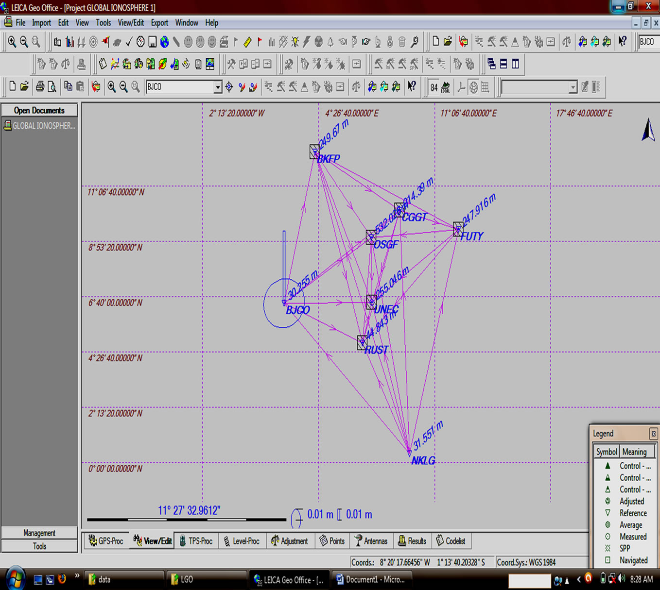 (a)
(a)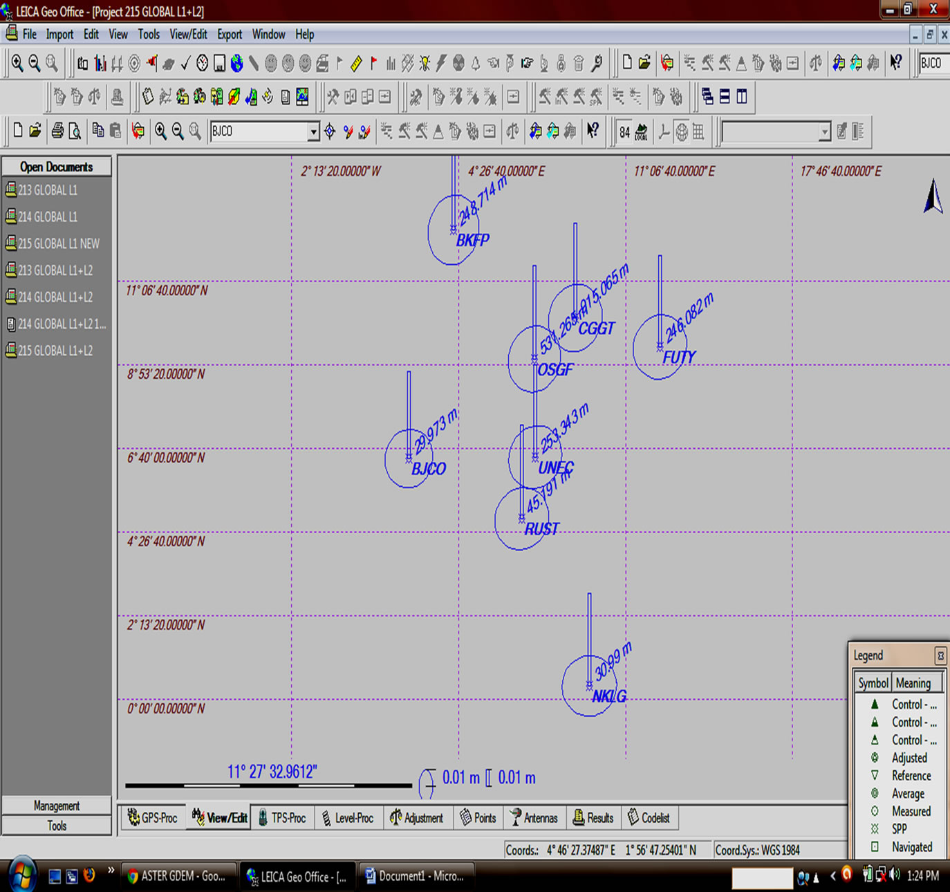 (b)
(b)
Figure 2. (a) Snapshot screen for relative network solution using dual frequency; (b) Snapshot screen for SFPPP.
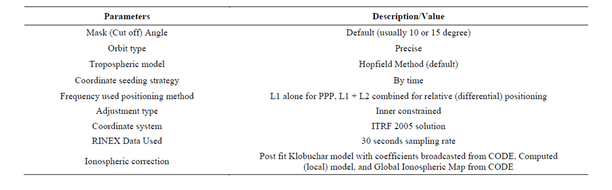
Table 1. Summary of processing parameter used in the study.
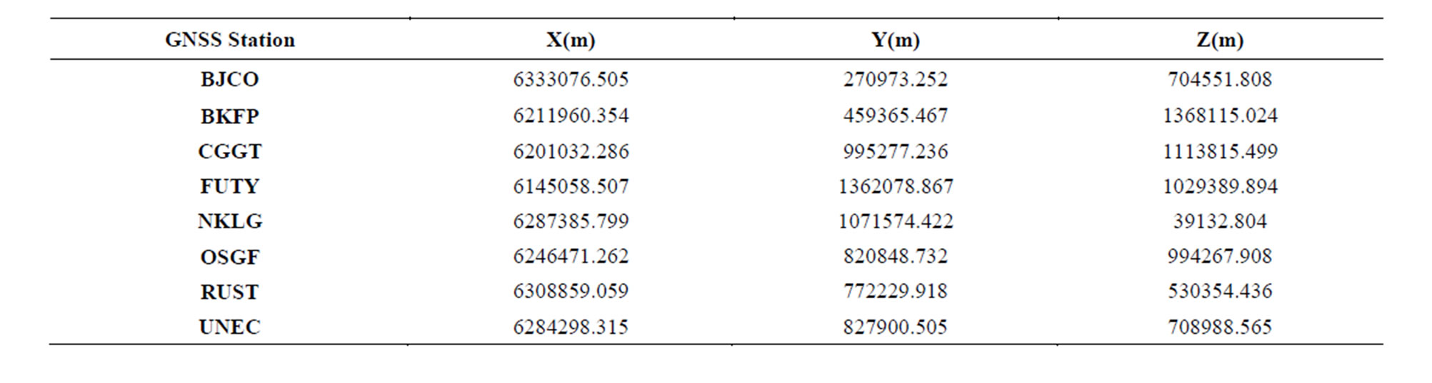
Table 2. Known ITRF coordinates of GNSS stations under investigation.
ance) check for gross error detection (outliers) which may have resulted from undetected cycle slip error or snooping. The 2RMS test was adopted for the quality control check (i.e., average difference ± 1.96 standard deviation of the difference), after all the station coordinates were subjected to the test, the mean (average) values for the days under investigation for the two different epochs are computed in Tables 3-7.
A statistical test was conducted to investigate the statistical agreement between the coordinate estimates from the different methods of ionospheric correction and the known ITRF solution of each station. The Bland-Altman plot [10,11] was used. The Bland-Altman plot, or difference plot, is a graphical method to compare two measurements techniques. In this graphical method, the differences (or alternatively the ratios) between the two techniques are plotted against the averages of the two techniques. Alternatively, according to Krouwer [12], the differences can be plotted against one of the two methods, if this method is a reference or “standard” method. As in this case, the known ITRF solutions of the station under investigation were considered as the reference method. Thirty (30) difference plots were generated for the two campaigns of observation; samples of the difference plot are presented in Figures 3-5. All computation was done using Analyse-it software, version 2.12.
The bias was also determined for each of the plots. The bias is the average difference between variables and should ideally be zero. Thus, near zero, values signify the agreement between the measurement technique and the standard method. Tables 8 and 9 show the biases for the different ionospheric mitigation approaches when compared with the reference (ITRF solutions).
From Tables 8 and 9, the biases in the (X, Y, Z) components for each approach can be considered as points in the Euclidean three space that deviate from the reference (Known ITRF solution) which has an assumed value of (0, 0, 0) for the three components. Thus the displacements from the reference or standard can be considered as the Euclidean distance between each of the approaches and the reference. figure 6 shows a plot of the displacements from the reference value, and the displacements were computed as the Euclidean distance between each approach and reference method. From Figure 6, it is evident that the effect of the ionosphere on position estimation can be severe if not corrected for, it can cause displacement of up to 7 m or more during intense ionospheric activities. The different mitigation approaches have all reduced the effect of the ionosphere in both epochs. The GIM from CODE proves to be a very efficient approach since it performs better than the DGPS approach in the two epochs of observation. Ideally, the DGPS is supposed to provide the best result, and the poor performance of the method can be attributed to the sparse of the network which has resulted in large inter-station distance. Generally, the results presented in figure 6
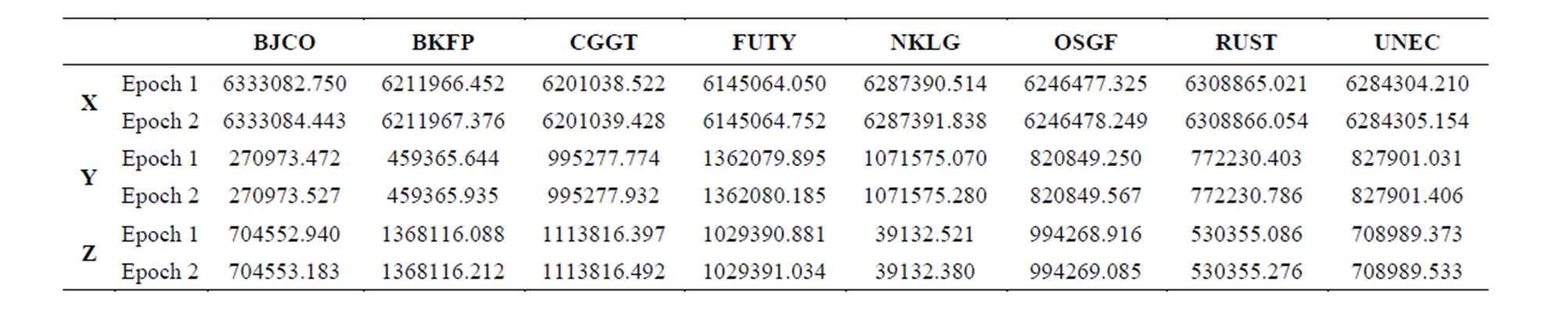
Table 3. Mean coordinates of GNSS stations estimated without ionospheric correction.
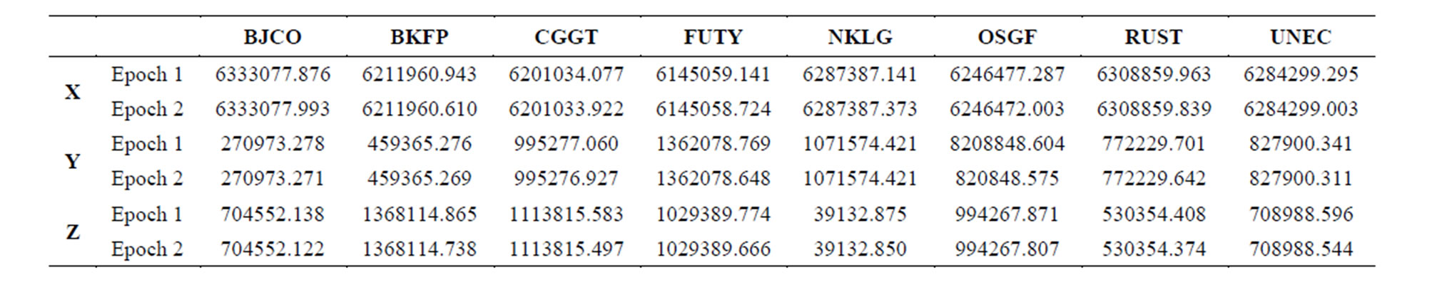
Table 4. Mean coordinates of GNSS stations estimated with the computed ionospheric correction.
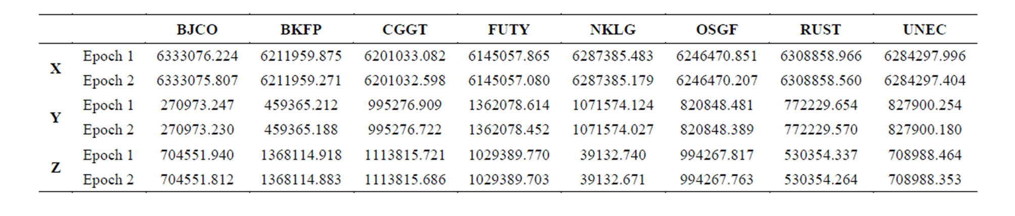
Table 5. Mean coordinates of GNSS stations estimated with GIM from CODE.
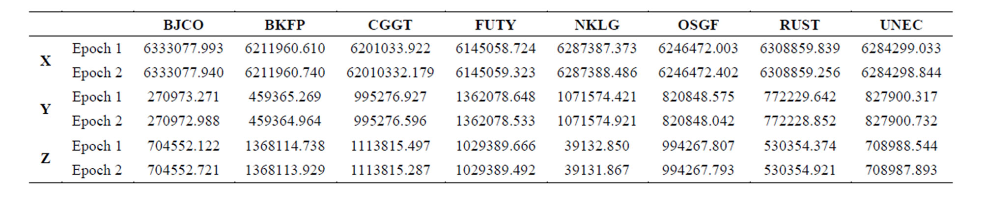
Table 6. Mean coordinates of GNSS stations estimated with the Klobuchar ionospheric correction model.
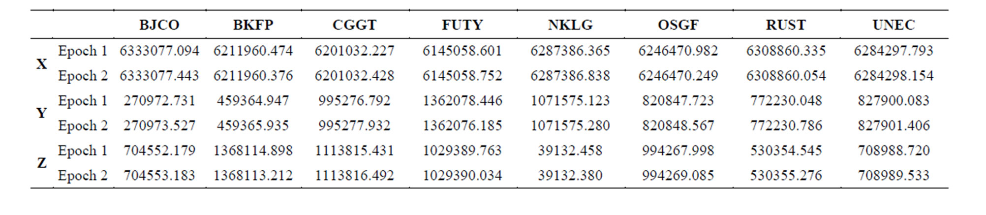
Table 7. Mean coordinates of GNSS stations estimated from dual frequency DGPS.
indicate a significant progress in the PPP mode of observation as it stands out to be very advantageous for user of networks or in a situation where no reference station is available.
Observational data, in addition to navigation and clock information from eight GNSS stations in the low equatorial region of West Africa, were processed using SFPPP technique. Different options for correcting for the effect
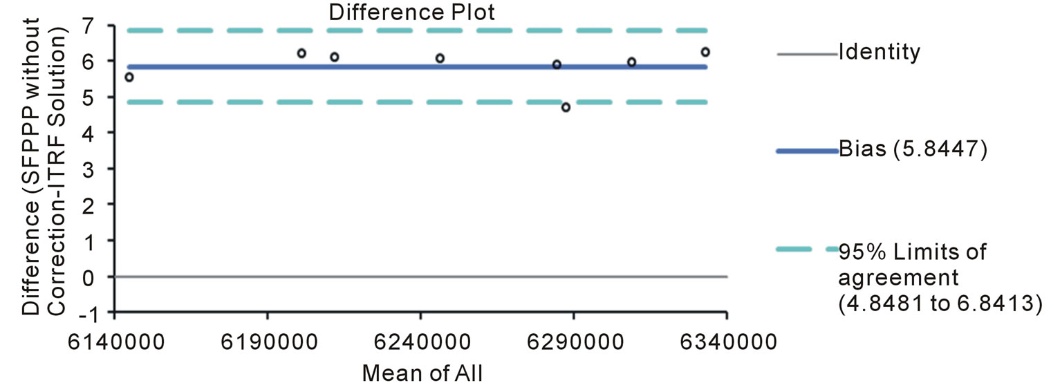
Figure 3. A sample of the Bland Altman plot (difference plot) depicting the bias when ionospheric correction was not applied at all the stations for epoch 1 (X-component).
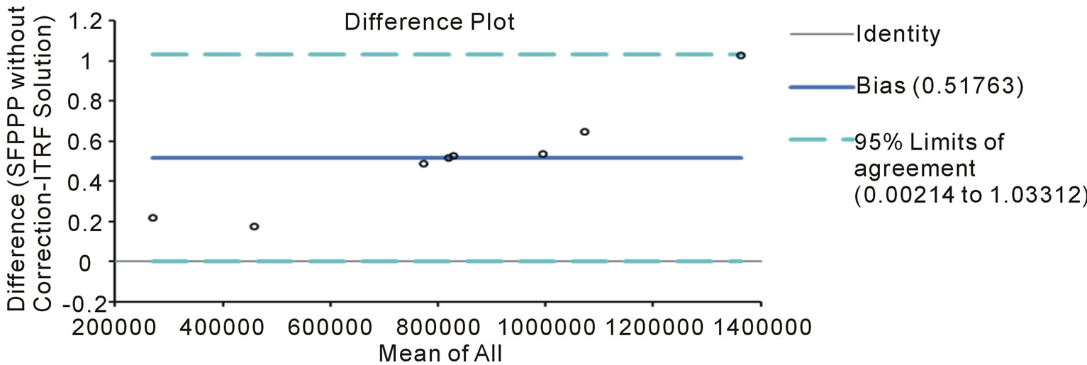
Figure 4. A sample of the Bland Altman plot (difference plot) depicting the bias when ionospheric correction was not applied at all the stations for epoch 1 (Y-component).
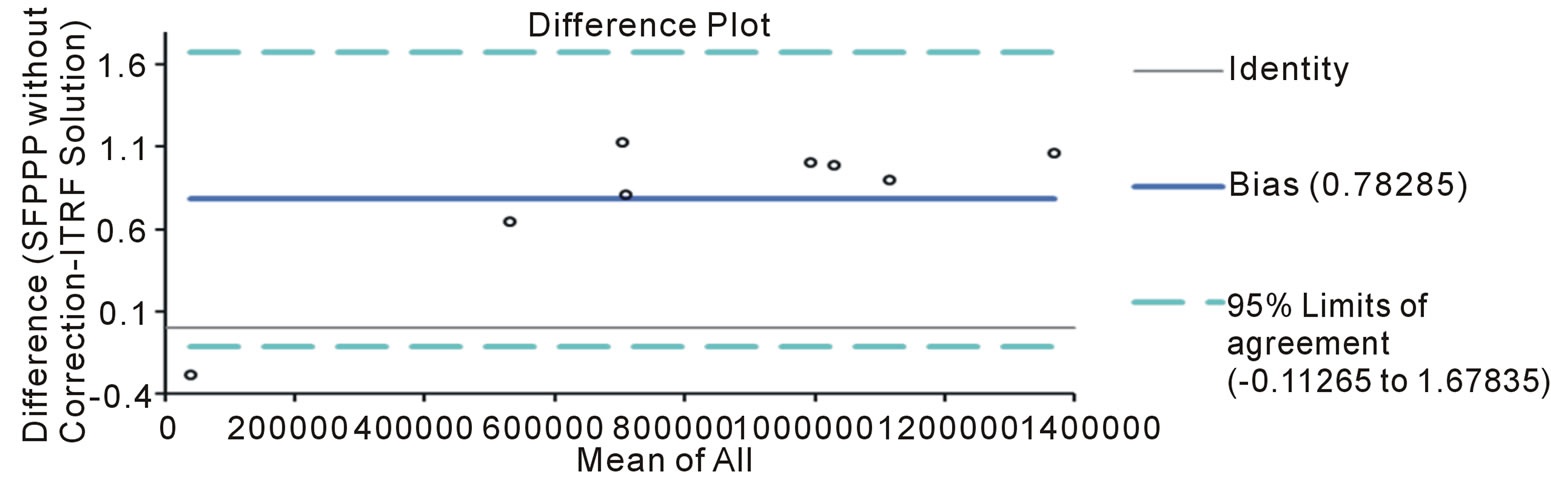
Figure 5. A sample of the Bland Altman plot (difference plot) depicting the bias when ionospheric correction was not applied at all the stations for epoch 1 (Z-component).
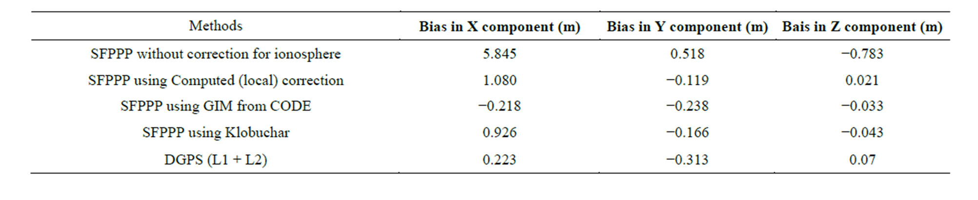
Table 8. Bias estimate for each approach (Epoch 1).
of the ionospheric were investigated to assess the positioning accuracy that can be achieved from SFPPP. The result of the study clearly demonstrates the significance of removing or correcting for the effect of the ionosphere. As it has been observed that some residual errors still remain in the estimated user position even after using dual frequency receivers in a relative approach. User of single frequency receiver for PPP only needs to understand
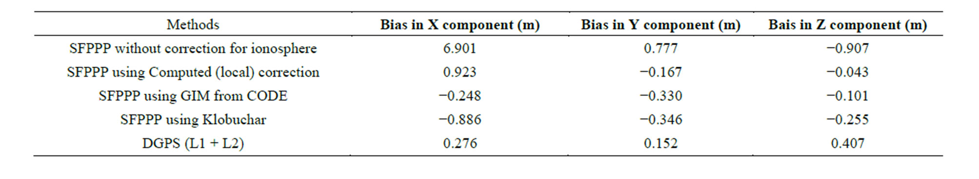
Table 9. Bias estimate for each approach (Epoch 2).
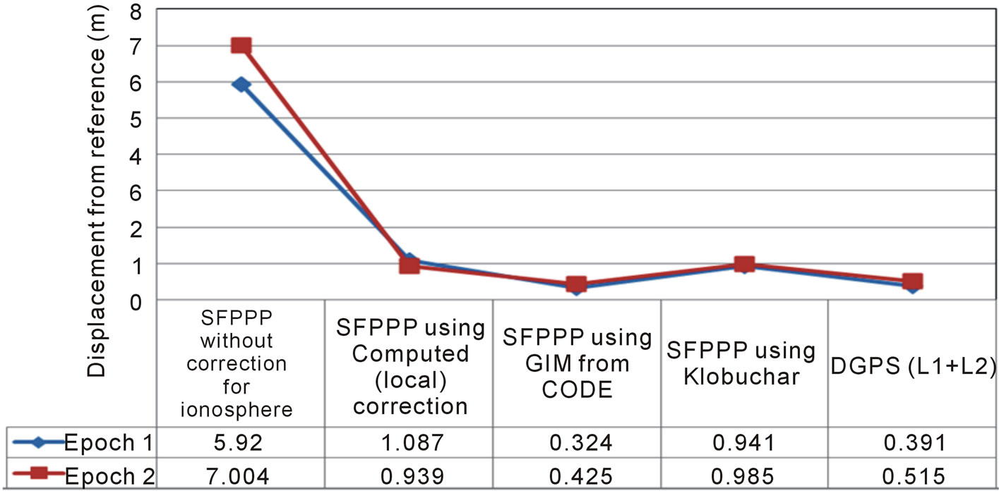
Figure 6. Displacement of stations from the reference based on ionospheric correction approach.
the behavior of the ionosphere at the time of their observation to attain acceptable limit of accuracy. It is believed that with expected improvements in satellite clock error bias estimation in the future, the accuracy of SFPPP will be greatly improved. As the results of this study have demonstrated, it will be of great importance if the accuracy of the different GIM produced by different organizations is compared and more effort should be made on the improvement of PPP algorithm to include effective modeling of clock errors and atmospheric effects. SFPPP can possibly replace the current widely used technique of relative DGPS in many applications, in view of the disadvantages of sparse networks and consequent long baseline errors associated with the DGPS technique. Finally, efforts are required to develop a RIM ionospheric model for the low equatorial African region and corrections from such are made available to users for Near Real Time (NRT) applications.
REFERENCES
- M. Abd-Elazeem, A. Farah and A. F. Farrag, “Assessment Study of Using Online (CSRS) GPS-PPP Service for Mapping Applications in Egypt,” Journal of Geodetic Science, Vol. 1, No. 3, 2011, pp. 233-239. http://dx.doi.org/10.2478/v10156-011-0001-3
- K. Huber, C. A. Heuberger, A. Karabatic, R. Weber and P. Berglez, “PPP: Precise Point Positioning-Constraints and Opportunities,” A Presentation at FIG Congress, Sydney, 11-16 April 2010.
- S. Choy, K. Zhang and D. Silcock, “An Evaluation of Various Ionospheric Error Mitigation Methods Used in Single Frequency PPP,” Journal of Global Positioning Systems, Vol. 7, No. 1, 2008, pp. 62-71.
- Y. Yuan, X. Huo and J. Ou, “Models and Methods for Precise Determination of Ionospheric Delay Using GPS,” Progress in Natural Science, Vol. 2, No. 17, 2007, pp. 187-196.
- ARINC Research Corporation, “GPS Interface Control Document ICD-GPS-200 (IRN-200C-004): Navstar GPS Space Segment and Aviation User Interfaces,” 2000.
- J. A. Klobuchar, “Ionospheric Time-Delay Algorithm for Single-Frequency GPS Users,” IEEE Transactions on Aerospace and Electronic Systems, AES, Vol. 23, No. 3, 1987, pp. 325-331.
- K. Chen and Y. Gao, “Real-Time Precise Point Positioning Using Single Frequency Data,” Proceedings of the ION GNSS 18th International Technical Meeting of the Satellite Division, Long Beach, 13-16 September 2005, pp. 1514-1523.
- CODE, “Global Ionosphere Maps Produced by CODE,” 2007. http://www.aiub.unibe.ch/content/research/gnss/code_research/igs/global_ionosphere_maps_produced_by_code/index_eng.html
- L. Geosystem, “Official Manual of Leica geooffice Software,” 2010. www.leica-geosystems.com
- J. M. Bland and D. G. Altman, “Statistical Methods for Assessing Agreement between Two Methods of Clinical Measurement,” Lancet, Vol. 327, No. 8476, 1986, pp. 307-310. http://dx.doi.org/10.1016/S0140-6736(86)90837-8
- J. M. Bland and D. G. Altman, “Measuring Agreement in Method Comparison Studies,” Statistical Methods in Medical Research, Vol. 8, 1999, pp. 135-160. http://dx.doi.org/10.1191/096228099673819272
- J. S. Krouwer, “Why Bland-Altman Plots Should Use X, Not (Y+X)/2 When X Is a Reference Method,” Statistics in Medicine, Vol. 27, 2008, pp. 778-780. http://dx.doi.org/10.1002/sim.3086