Received 12 May 2016; accepted 9 July 2016; published 12 July 2016

ABSTRACT

It is well known that the boundary element method (BEM) is capable of converting a boundary- value equation into its discrete analog by a judicious application of the Green’s identity and complementary equation. However, for many challenging problems, the fundamental solution is either not available in a cheaply computable form or does not exist at all. Even when the fundamental solution does exist, it appears in a form that is highly non-local which inadvertently leads to a system of equations with a fully populated matrix. In this paper, fundamental solution of an auxiliary form of a governing partial differential equation coupled with the Green identity is used to discretize and localize an integro-partial differential transport equation by conversion into a boundary-domain form amenable to a hybrid boundary integral numerical formulation. It is observed that the numerical technique applied herein is able to accurately represent numerical and closed form solutions available in literature.

Keywords:

Boundary Element Method, Green’s Identity, Complementary Equation, Fundamental Solution, Hybrid Formulation, Integro-Differential Transport Equation

1. Introduction

The governing equation for a convective-dispersive transport phenomenon is given by:

(1)

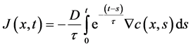
where c is concentration; v is the flow velocity; is the dispersive tensor; t is the time variable and is the rate of solute mass exchange. Equation (1) yields satisfactory results in controlled environments in the absence of media heterogeneities. However, it exhibits certain limitations in modeling real life phenomenon. Its deviation from Fickian theory, results in an infinite speed of propagation of the scalar field (Cattaneo [1] Curtin and Pipkin1 [2] , Ferreira and Oliveira [3] , Hristov [4] ). In order to overcome this unphysical property, Fick’s law is replaced by a flux accompanied by a memory term. It was proposed (Cattaneo’s [1] ) that the flux at a certain point x and at time t should be a consequence of scalar variation at some point x but after an elapsed time. Based on this, Ficks equation is modified to read:

(2)

where is a delay parameter. Applying a first order Taylor series expansion to the flux we obtain the so-called Cattaneo’s flux term.

(3)

Without any loss in generality, Equation (1) can be recast to read

(4)

where are the reaction and source/sink terms. The source/sink term accounts for the injection or extraction of mass into or out of the system. are the diffusion coefficient and velocity variables. The term inside the integral term accounts for the memory of the system. Equation (4) is a one-dimensional integro-partial differential equation which describes the transport of quantities such as heat, vorticity, energy and mass and is very important in many physical systems especially those involving the environment. It comes with the following constraints.

An initial condition of the type

(5)

and boundary conditions

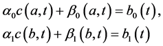(6)

where. In addition, are given constants.

Fundamental solutions generated from “free-space” Greens functions are usually applied in boundary integral analysis of transport equations. Efforts to make them more applicable to boundary element method (BEM) formulation, especially for non-homogeneous material, can be found in (Shaw [5] ) and (Shaw and Manolis [6] ). These have not only met with mixed results but have also been found to be inadequate for a good number of problems of engineering interest.

For example, adopting the classical boundary element approach to viscoelastic materials or to cases which incorporate the memory term requires fundamental solutions that are yet not well known except for the simple Maxwell material whose analytical solution is available (Gaul and Schanz [7] ). Numerical attempts to deal with this include that of Schanz and Antes [8] . They studied a BEM viscoelastic formulation based on the so called convolution integral method proposed by Lubich [9] in 1988. In this work, a quadrature formula whose weights are determined by the Laplace transform of the fundamental solution is applied to evaluate a convolution inte- gral and the entire formulation numerically handled by a multi-step procedure.

The hybrid boundary-integral-finite element procedure adopted herein employs the Green’s function of the Laplace operator, and retains the time marching feature of classical BEM, but its spatial discretization enlists a local support feature that is similar to that of the finite element. This guarantees some attractive outcomes; it facilitates the hybridization process especially for schemes that are element or nodal based (Onyejekwe [10] [11] ) and establishes a hybrid computational method which exploits the strengths of its composite parts. This is the key motivation for this study.

2. Numerical Formulation

A typical boundary integral discretization requires both the complementary differential equation and the free- space Green’s function.

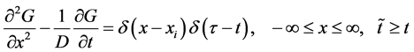(7)

(8)

where is the source node and x is the field node and by the same token both t and represent the source and field nodes in the temporal coordinates. The flexibility offered by a hybridization procedure allows the integral kernel in equation (4) to be evaluated at each node.

We consider defined in the region where

(9)

and

(10)

We adopt a composite weighted trapezoidal rule in the temporal coordinate for the memory term.

(11)

Equation (4) is finally converted to its integral analog by the Green’s second identity to yield:

(12)

where are given and I is the “memory” or the hereditary’ term; can be a constant or a function of

the dependent variable,

This hybrid formulation unlike a typical boundary integral formulation requires that the computational domain be discretized into elements over which the scalar variable will assume some functional distributions. This is represented for the dependent variable as

(13)

where represents the current time level, while denotes previous time level. and are interpolating functions in space and time respectively. The element equation can now be written as:

(14)

Equation (14) is put in a compact matrix form

(15)

3. Numerical Test Examples

Example 1 Consider the following special case of Equation (4) with reaction term of the nonlinear variety (Khuri and Sayfy [12] ),

(16)

where subject to the initial condition

(17)

and boundary conditions

(18)

Next we account for the source term where

(19)

The exact solution is given by

(20)

The numerical solutions are obtained with respectively. The closeness of Figure 1 to that of Khuri and Sayfy [12] and the magnitude of absolute errors as a result of comparison between analytic and numerical results in Table 1 demonstrate the reliability of the numerical formulation developed herein.

Example 2 We consider a special case of Equation (4) given by:

(21)

At time = 0.025000, L2-Norm = 0.000178, L-Infinity Norm = 0.000463, Root Mean Square Error = 0.000899.

where, are the velocity and diffusion coefficient s respectively.

The initial and boundary conditions are given as:

(22)

(23)

Equation (21) is a transport equation that involves a convective-diffusive process coupled with a memory term. It is one of the most important equations of mathematical physics and has been used to describe the transport of such quantities like mass, heat, vorticity, energy and momentum. In the absence of the memory term, the analytical solution can be determined by method of separation of variables. This is expressed as:

(24)

The numerical solution has been found to develop a steep front or boundary layers at x = 1 (Feng and Tian 2006). Profiles of the numerical solution of equation (21) and the corresponding analytical solution without the memory term (equation (24)) are displayed in Figure 2(a) and Figure 2(b) for the following problem parameters:. While some instabilities can be detected in Figure 2(b), none can be found in 2a. This confirms an earlier work by Feng and Tian [13] . In addition, this observation validates the

interesting physics brought to play by the introduction of the memory term in the C-D equation. The modification of the flux term which takes care of the infinite speed of species propagation introduces an additional diffusion term. Again a close look at Equation (21) shows that we have two elliptic operators whose second order derivatives are multiplied by positive parameters. These derivatives model the diffusion process while the only first order derivative is associated with the convective process. Diffusion has always been known to play a significant role in the region of rapid changes (the boundary layers) where the scalar profile exhibits a steep profile. When a standard numerical procedure is applied to a C-D problem, if the diffusion term is relatively smaller than the convective term, the computed solution profile is often oscillatory. Whereas if there exists an “excess” (superfluous) diffusion term, the computed profile is smeared as demonstrated in Figure 2(a). It will also be interesting to compare the effects on the scalar profiles introduced by different magnitudes and discretizations of the convection term. However, the details of this will be the theme of a forthcoming paper.

4. Conclusion

The main thrust of this paper is a seamless incorporation of non-Fickian flux and memory into a localized element-based boundary element method. The advantage of this technique lies in the possibility of admitting realistic experimental information into a governing differential equation without complicating BEM formulation. For example, it offers a feasible alternative for applying BEM to describe transport processes in viscoelastic media where the inclusion of memory term is vital.

Cite this paper

Okey Oseloka Onyejekwe, (2016) A Domain-Boundary Integral Treatment of Transient Scalar Transport with Memory. Applied Mathematics,07,1241-1247. doi: 10.4236/am.2016.711109

References

- 1. Cattaneo, C.S. (1948) Conduzione del calore, Atti del. Seminario Matematico e fisico dela Universita di Modena, 3, 3-21.
- 2. Curtin, M.E. and Pipkin, A.C. (1968) A General Theory of Heat Conduction with Finite Wave Speeds. Archive for Rational Mechanics and Analysis, 31, 113-126.
http://dx.doi.org/10.1007/BF00281373 - 3. Ferreira, J.A. and de Oliveira, P. (2007) Memory Effects and Random Walks in Reaction-Transport Systems. Applicable Analysis, 86, 99-118.
http://dx.doi.org/10.1080/00036810601110638 - 4. Hristov, J.A. (2013) Note on the Integral Approach to the Nonlinear Heat Conduction with Jeffrey’s Fading Memory. Thermal Sciences, 17, 733-737.
- 5. Shaw, R.P. (1994) Green-Functions for Heterogeneous Media Potential Problems. Engineering Analysis with Boundary Elements, 13, 219-221.
http://dx.doi.org/10.1016/0955-7997(94)90047-7 - 6. Shaw, R.P. and Manolis, G.D. (2000) Elastic Waves in One-Dimensionally Layered Heterogeneous Soil Media. Adv. EarthQ, 5, 215-246.
- 7. Gaul, L. and Schanz, M. (1992) BEM Formulation in time Domain for Viscoelastic Media Based on Analytical Time Integration. In: Brebbia, C., Dominguez, J. and Paris, F., Eds., Boundary Elements XIV, Vol. 2, Computational Mechanics Publications, Southampton, 223-234.
- 8. Schanz, M. and Antes, H. (1997) Application of Operation Quadrature Methods in Time Domain Boundary Element Methods. Meccanica, 32, 179-186.
http://dx.doi.org/10.1023/A:1004258205435 - 9. Lubisch, C. (1988) Convolution Quadrature and Discretized Operational Calculus. Numerische Mathematik, 52, 129-145.
- 10. Onyejekwe, O.O. (2014) The Effect of Time Stepping Schemes on the Accuracy of Green Element Formulation of Unsteady Transport. Journal of Applied Mathematics and Physics, 2, 621-633.
- 11. Onyejekwe, O.O. (2015) A Hermitian Boundary Integral Hybrid Numerical Formulation for Nonlinear Fisher-Type Equations. Applied and Computational Mathematics, 4, 83-99.
- 12. Khuri, S.A. and Sayfy, A. (2009) A Numerical Approach for Solving an Extended Fisher-Kolmogorov-Petrovskii-Piskunov Equation. Journal of Computational and Applied Mathematics, 233, 2081-2089.
- 13. Feng, X.F. and Tian, Z.F. (2006) Alternating Group Explicit Method with Exponential-Type for the Diffusion Convection Equation. International Journal of Computer Mathematics, 83, 765-775.
http://dx.doi.org/10.1080/00207160601084463