ABSTRACT

The paper Connecting Newton’s G With the Rest of Physics-Modern Newtonian Gravitation Resolving the Problem of “Big G’s” Value derived the value of the gravitation constant “Big G”, G of Newton’s Law of Gravitation, directly from other physics fundamental constants but left it to a subsequent paper to experimentally validate the derived G. The present paper performs that validation by examining various past experiments intended to measure “Big G”, in each case determining the acceleration, a_g, as found per Einstein’s General Theory of Relativity versus per Modern Newtonian Gravitation for that case. The ratio of those two times the reported measured “Big G” value yields a result identical to the G determined from the derived formulation for G, within the error range of the reported measured “Big G” measurement. That thus validates the correctness of the derived formulation for G. The next important issue, what causes gravitation, how does the effect take place, is addressed and resolved in the paper The Mechanics of Gravitation-What It Is; How It Operates, which is available in this journal.

Keywords:

Gravitation, Newton’s “Big G”, Fundamental Constants

1. Introduction and Summary

The theory of gravitation presented by General Relativity [GR], although highly successful at treating phenomena resulting from gravitation, fails to obtain precise measurement of “Big G”, the Newtonian constant of gravitation, has failed to connect “Big G” to the rest of physic’s fundamental constants, proffers no cause or mechanism for the operation of gravitation, and consequently prevents any development of means of controlling or modifying gravitation. The Modern Newtonian [MN] theory of gravitation overcomes all of those GR failures.

The difference between the two theories is in the interpretation of Newton’s formula for gravitational action, Equation (1) below, specifically the interpretation of the.

(1)

In GR the separation distance, d, between the gravitating objects’ masses, M and m, is the distance between the centers of the two.

In MN each of the objects is composed of myriad particles, atoms, each of which performs Equation (1) between itself and each of the particles in the other object, individually, one-on-one as an independent pair. Each such pair has its particular separation distance. The inverse separation distance squared, 1/d², of Equation (1) is the overall average of the myriad individual inverse separation distances squared, corrected to the vector component parallel to the centerline between the objects, Avg [1/d²].

To convert a measurement of “Big G” done using the GR version of Equation (1) to the value that would have been obtained if the measurement had been done using the MN version of Equation (1) it is only necessary to multiply the GR version measurement by the GR inverse separation distance squared, 1/d², divided by the MN average of the squared inverse separation distances, Avg [1/d²].

The paper Connecting Newton’s G With the Rest of Physics-Resolving the Problem of “Big G’s” Value [1] presents a formula for calculating “Big G” from other fundamental physics constants. From that the correct value of “Big G” is 6.636046823 × 10⁻¹¹ m³・kg⁻¹・s⁻². In converting GR “Big G” measurements to MN the GR are not precise due to their various measurement errors so that those converted to MN per the above procedure will not arrive at the above precise “Big G” from fundamental constants but will deviate because their other measurement errors will still be present.

The results of some such conversions, from GR to MN, are presented in Table 1. Note the variations in the “Corrected” values around the “Big G from fundamental constants” 6.636046823 × 10⁻¹¹ value. The variations in the “Corrected” are caused by the original measurements’ variations.

The conclusion is that the cited paper and its formulation for “Big G” in terms of other fundamental physics constants is valid and correct. That which GR could not produce has been produced and resolved by MN gravitation which consequently must supersede GR gravitation.

Further, this MN validation also “legitimizes” the Gravito-Electric Power Generation and the Gravitation Deflection Deep Space and Planet Surface Flying Vehicle Drive proposed in the paper Gravitational and Anti-Gravitational Applications [2] which applications should be tested.

2. On the Theory of Measuring “Big G”

There is only one universal correct value of “Big G”. Except for various errors

All data in SI units: meters, kilograms, seconds. * = ×10⁻¹¹. Newton’s Law of Gravitation is. That, with Law of Motion, F = m∙a, is. Measurement = which experiment. D = spheres center-to-center separation distance. GR = General Relativity calculation of gravitation, 1/d² = 1/D². AvgD = Calculated average of parallel-to-centerline-components of reciprocal separation distances squared is 1/d². MN = Modern Newtonian calculation of gravitation using AvgD. Gm = reported measured “Big G”. Gc = Gm・[GR/MN] = Gm・[1/D²/AvgD]. G from its relation to other fundamental constants = 6.636046823 × 10⁻¹¹.

and inaccuracies in conducting the measurement every measurement must provide that exact same result. While the gravitational acceleration or force acting between objects varies according to Newton’s Law that variation is due to varying values of the masses involved and the separation distance not the value of “Big G” which is a fixed constant.

But, in the MN conception of the operation of Newton’s Law the separation distance is not the simple distance between the centers of the two gravitating masses; it is the average of the inverse square separations particle to particle, one on one, of all of the particles making up the masses. Therefore different configurations of the gravitating masses produce different gravitational acceleration and force for the same GR values of the masses with the same GR center to center separations.

Nevertheless, whatever the values of the masses are and whatever the configuration of their particles and whatever the resulting gravitational acceleration and force, the measurement of “Big G” must produce the same universal value. Any deviations or discrepancies from the correct value can only be due to measurement errors and inaccuracies.

Consider two measurement alternatives both having the same masses acting and the same GR separation distance between the centers of those masses, but the configurations of the MN interacting particles making up the masses are different. For example, alternative #1 is two spheres whereas alternative #2 is two cylinders.

It might be thought that the measured gravitational acceleration or force would be the same for the two alternatives because in the GR conception of Newton’s Law of Gravitation the two alternatives are identical, not a little different. But regardless of the GR thinking, the actual measurements will be different because it is the MN gravitational action that operates, always.

The MN average inverse square separation, Avg [1/d²], in the two alternatives must be at least a little different. The MN difference in the two alternatives will produce accordingly different resulting gravitational acceleration or force which will result in accordingly different values for “Big G” calculated by GR.

The formula for correcting those GR values of “Big G” to the MN values for the two alternatives results in the same value for “Big G” always.

(2)

In both alternatives the formula cancels out the GR 1/d² [used to calculate “Big G” from the actually measured gravitational acceleration or force observed] replacing it with the [Avg [1/d²]] that was actually operating when the measurement was made.

The problem in making this correction is to accurately calculate Avg [1/d²], that is to exactly reproduce the particle-by-particle, particle-to-particle, one-on- one action that actually operates in the Newtonian gravitational interaction, that actually operated in each experimental result to be converted.

3. The Point-on-Point Gravitational Interaction between Objects

In this “Big G” Calculation, each of the particles in M is paired, one at a time, with every particle in m. The particle-to-particle separation distance in their 3-dimensional space is determined from the 3-dimensional Law of Pythagoras. That distance is then squared and its reciprocal taken producing the equivalent of gravitation’s 1/d². corresponding to the contribution to f_grav of the particular particle pair of one particle of M interacting with one particle of m. The components of this gravitational action that are perpendicular to the center-to-center line have no net effect because over all of the particle-to-particle interactions and the symmetry of the configuration they cancel out. Only the component of the gravitational action between two particles that is parallel to the center-to-center line is effective gravitation. That component is evaluated by projecting the 3-dimensional line of each particle-to-particle interaction onto the center-to- center line.

The average of the accumulation of all of these [MN] particle-to-particle results is then compared to the corresponding [GR] center-to-center results.

This calculation is part of the calculating of the particle-on-particle interactions between the particles of a “source” gravitating object and the “encountered” gravitating object the particles represented by approximating samples [dealing with “points” is impossible; there are an infinite number]. The objects are deemed monolithic solids of purely one kind of particle. The particles are expressed in terms of a set of 3-dimensioning axes: x, y, and z.

The origin of those coordinates is at the center of the source object. The coordinates are xs, ys, and zs designating individual points in the source object. For the purpose of referring to particles in the encountered object a secondary origin is taken at the center of that object and the coordinates there are xe, ye, and ze.

The center-to-center (origin-to-origin) separation distance of the two objects is the distance D. In terms of source dimensioning the origin of the encountered object is located at xs = −D. Any encountered coordinate designation is referred to the source dimensioning by adding “−D” to the xe dimension.

The total particle-on-particle interaction is obtained by summing the individual contributions of each source point interacting with each encountered point. The scanning process selects successive values of zs, each value representing a 2-dimensional “slice” of the source object. The slice is then scanned into successive values of ys representing 1-dimensional lines making up the slice. Each line is then scanned into successive values of xs representing 0-dimensional points making up the line.

Each of those source points then interacts with each of the points of the encountered object selected by the same slice-line-point type of scanning process as used for the source object. When the currently selected source point i, which is zs_i, ys_i xs_i, has interacted with every one of the encountered object points successively one at a time then the scan proceeds to source point (i + 1) and its interaction with every one of the encountered object points.

The entire process is extremely lengthy. To shorten it, which corresponds to speeding it up, the portion of the process that is most used, the xe scan, is replaced by developing a formula that gives the same result as the xe scan it replaces. This procedure has two advantages, the first being that calculating the effect of an entire line of points “in one fell swoop” is much faster than calculating that entire line one point at a time.

The second advantage is as follows. There are an infinite number of points in a line and they cannot be individually addressed. Rather the line must be divided into a number of sequential identical segments they being samples of the line. The more segments the line is represented by the greater the precision of the samples accurately representing the line. The replacement of xe sampling with “one fell swoop” calculation also produces the maximum precision.

The same necessity for sampling applies to the succession of lines as the ye- variable progresses and to the succession of “slices” as the ze-variable progresses. Therefore each sample “point” is actually a sample volume, a cuboid (or rectangular parallelepiped) of which the “point” is the location of the cuboid center and which cuboids all taken together are the volume of the object.

A spherical quadrant is each of four parts of a sphere divided by two planes at right angles to each other. In the present 3-dimensional x, y, z coordinate system let the two planes be the x-y plane and the x-z plane as in Figure 1 and Figure 2 below. Taking advantage of the symmetry of the two spheres addressing each other along a line connecting their centers as in the right figure below, that center line their common x-axis, each sphere has four such quadrants and if the entire source sphere is scanned then, because of the symmetry, each of the encountered sphere’s four quadrants produces the same effect and only one of them need be scanned.

Furthermore, the source sphere need be scanned in only one of its four quadrants, that involving +ys and +zs the other three quadrants being selected by successively choosing −ys with +zs, −ys with −zs, and +ys with −zs.

Finally because of the symmetry the interaction of Q1 with Qb is the same as Q1 with Qc so that only one of those two need be calculated, the result of that being doubled.

The xe scan is for one single point of the source sphere, that is one single set of values for xs, ys, and zs. It is for one single line parallel to the x-axis, that line for one single set of values of ye and ze, the scan replacing sampling values of xe with a single overall value for that line calculated by integration.

The above simplification due to quadrants symmetry applies also to any non-spherical form so long as it is symmetrical relative to the x-axis.

4. The X-Scan Integral

4.1. Developing the Integrand

The quantity to be calculated is Avg [1/d²], by the accumulation of Incr [below] over the entire scan as follows.

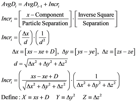(3)

(4)

In terms of the variable of integration, xe, [x below] and relative to its “encountered” origin the range of the xe scan excursion is:

from to (5)

but, the overall integration is in the source frame of reference and the range must so be. Therefore, the range is from to.

The integral is then:

(6)

where for scanning a single encountered x-line for a single source point [at zs, ys, xs] the encountered ze and ye are constants. The only variable is xe as x.

The above derivation assumes the spheres case as in Figure 1; however, the same general procedure applies to any form having the same x-axis symmetry. The only modification needed is the range of the integration.

4.2. Evaluating the Integral

To integrate a function containing the procedure is to make the substitution: x² + K = y² from which x² = y² − K and 2x∙dx = 2y∙dy. The above integrand then transforms as follows:

(7)

The right hand expression of the integrand integrates as follows.

Reverting back through the substitution to a function of x:

But, this and is a constant relative to integrating on x. Further x is [xs − xe + D] where xe is the variable and xs a constant; therefore:

(8)

5. Scanning and Calculating the X-Scan Integral

The remaining procedure is to calculate the above evaluated integral in conjunction with scanning the M and m objects. Appendix B is a Basic Language program for performing the scanning and calculating the x-scan for each pair of particles selected.

6. Comprehensive Gravitation

This paper is an essential integral part of a set of papers treating Comprehensive Gravitation. The papers of the set are listed in references [1] [2] [3] [4] [5] .

References^*

[1] Ellman, R. (2016) Connecting Newton’s G with the Rest of Physics―Modern Newtonian Gravitation Resolving the Problem of “Big G’s” Value. ResearchGate. https://www.researchgate.net/profile/Roger_Ellman/info

[2] Ellman, R. (2016) Gravitational and Anti-Gravitational Applications. ResearchGate. https://www.researchgate.net/profile/Roger_Ellman/info

[3] Ellman, R. (2016) Comprehensive Gravitation. ResearchGate. https://www.researchgate.net/profile/Roger_Ellman/info

[4] Ellman, R. (2016) The Experimental Data Validation of Modern Newtonian Gravitation over General Relativity Gravitation. ResearchGate. https://www.researchgate.net/profile/Roger_Ellman/info

[5] Ellman, R. (2016) The Mechanics of Gravitation―What It Is; How It Operates. ResearchGate. https://www.researchgate.net/profile/Roger_Ellman/info

Appendices

A-Summary of Tests Results

B-A Sample Typical Basic Program File: Luther.bas.

C-“Big G” Calculation Basic Program Flow Diagram

D-Comparison of Parameters

Appendix A: “Big G” Calculation Tests Summary of Tests Results

Experiments Calculated

H. Cavendish, 1798, Wikipedia, “Cavendish Experiment”

R. Rose et al., 1969, “Determination of the Gravitational Constant G” PRL (21)12.

G. Luther & W. Towler, 1982, “Redetermination of the Newtonian Gravitational Constant G” PRL (48) 3.

C. Bagley & G. Luther, 1997, “Preliminary Results of a Determination of the Newtonian Constant of gravitation: …” PRL (78) 16.

J. Gundlach & S. Merkowitz, 2000, “Measurement of Newton’s Constant Using a Torsion Balance with Angular Acceleration Feedback”, PRL (85) 14.

St. Schlamminger et al., 2006, “Measurement of Newton’s Gravitational Constant”, Physical Review D of APS, 74

T. Quinn et al., 2013, “Improved Determination of G Using Two Methods”, PRL 111, 1011021 (2013).

Experiments Not Calculated Because of Insufficient Dimensional Data

P. Heyl, 1930, “A Redetermination of the Constant of Gravitation”, NIST Archives.

P. Heyl & P. Chrzanowski, 1942, “A New Determination of the Constant of Gravitation”, NIST Archives.

M. Fitzgerald & T. Armstrong, 1995, IEEE Archives.

W. Michaelis et al., 1995, “A New Precise Determination of Newton’s Gravitational Constant”, Metrologia of IOP.

J. Schurr et al., 1998, “Gravitational Constant Measured by Means of a Beam Balance”, PRL of APS.

F. Nolting et al., 1999, “Determination of G by Means of a Beam Balance”, IEEE archives.

T. Armstrong & M. Fitzgerald, 2003, “New Measurement of G Using the Measurements Standards Laboratory’s Torsion Balance”, PRL of APS.

L.-C. Tu et al., 2010, “New Determination of the Gravitational Constant G with Time-of-Swing Method” Physical Review D of APS, 82 (022001) and J.Luo et al., 2009, “Determination of the Newtonian Gravitation Constant with Time of Swing Method”. PRL 102, 240801.

H. Parks & J. Fuller, 2010, “Simple Pendulum Determination of the Gravitational Constant”, PRL of APS.

L.-C. Tu et al., 2010, “New Determination of the Gravitational Constant G with Time-of-Swing Method” Physical Review D of APS, 82 (022001) and J.Luo et al., 2009, “Determination of the Newtonian Gravitation Constant with Time of Swing Method”. PRL 102, 240801.

H. Parks & J. Fuller, 2010, “Simple Pendulum Determination of the Gravitational Constant”, PRL of APS.

Appendix B: A Sample Typical Basic Program File: Luther. Bas

This program is a sample typical of the programs used for calculating the various experiments. It was prepared and run using the PowerBASIC Consol Compiler Integrated Development Environment (IDE) version 6.03 from PowerBASIC Inc.

FUNCTION PBMAIN

1 REM BIG G INTEGRATION CALCULATION BASIC PROGRAM

CONSOLE.PRINT "METHOD = SPHERE TO SPHERE"

CONSOLE.PRINT "EXPERIMENT = LUTHER"

CONSOLE.PRINT ""

CONSOLE.PRINT "START: DATE = "; DATE$, " TIME = "; TIME$

BD$ = DATE$

BT$ = TIME$

10 REM OVERALL INITIALIZING

DIM COUNT AS DOUBLE

COUNT = 0

DIM AVGD AS DOUBLE

AVGD = 0

DIM N AS DOUBLE

N = 100

20 REM OVERALL INPUTTING

DIM RS AS SINGLE

DIM RE AS DOUBLE

DIM SEPD AS DOUBLE

DIM GM AS DOUBLE

RS = 0.0508255

RE = 0.0029

SEPD = 0.07029727

GM = 6.6726E-11

DIM JS AS DOUBLE

DIM JE AS DOUBLE

JS = RS / N

JE = JS / 10

30 REM INITIALIZE SOURCE SCAN - ZS CYCLE

DIM ZSF AS DOUBLE

ZSF = RS - JS / 2

DIM ZS AS DOUBLE

ZS = -JS/2

40 REM START NEXT SOURCE Z CYCLE

ZS = ZS + JS

50 REM INITIALIZE SOURCE Y CYCLE

DIM YSF AS DOUBLE

YSF = (SQR(RS^2 - ZS^2))-JS/2

DIM YS AS DOUBLE

YS = -JS/2

55 REM DISPLAY

IF COUNT > 0 THEN

CONSOLE.PRINT "1 OVER SEPD^2 = "; 1 / (SEPD ^ 2), "AVGD = "; AVGD / COUNT

CONSOLE.PRINT "ZS = "; ZS, " OUT OF ZSF = "; ZSF

CONSOLE.PRINT " "

END IF

60 REM START NEXT SOURCE Y CYCLE

YS = YS + JS

70 REM INITIALIZE SOURCE X CYCLE

DIM XSF AS DOUBLE

XSF = (SQR(RS^2 - ZS^2 - YS^2))-JS/2

DIM XS AS DOUBLE

XS = -(SQR(RS^2 - ZS^2 - YS^2))-JS/2

80 REM START NEXT SOURCE X CYCLE

XS = XS + JS

100 REM INITIALIZE ENCOUNTERED SCAN - ZE CYCLE

DIM ZEF AS DOUBLE

ZEF = RE - JE / 2

DIM ZE AS DOUBLE

ZE = -JE/2

110 REM START NEXT ENCOUNTERED Z CYCLE

ZE = ZE + JE

120 REM INITIALIZE ENCOUNTERED Y CYCLE

DIM YEF AS DOUBLE

YEF = (SQR(RE^2 - ZE^2))-JE/2

DIM YE AS DOUBLE

YE = -JE/2

130 REM START NEXT ENCOUNTERED Y CYCLE

YE = YE + JE

170 REM XE CALCULATION BY FORMULA

DIM CUMINCR AS DOUBLE

CUMINCR = 0

DIM RAD AS DOUBLE

RAD = (RE ^ 2 - ZE ^ 2)

IF RAD > YE ^ 2 THEN

RAD = SQR(RAD - YE ^ 2)

ELSE

RAD = 0

GOTO 200

END IF

DIM TAIL AS DOUBLE

TAIL = XS + SEPD + SEPD

DIM BALNC AS DOUBLE

BALNC = (YS - YE) ^ 2 + (ZS - ZE) ^ 2

DIM FIRST AS DOUBLE

FIRST = 1 / (2 * RAD)

DIM PIECEA AS DOUBLE

PIECEA = (RAD + TAIL) ^ 2

DIM SECOND AS DOUBLE

SECOND = 1 / SQR(PIECEA + BALNC)

DIM PIECEB AS DOUBLE

PIECEB = (-RAD + TAIL) ^ 2

DIM THIRD AS DOUBLE

THIRD = 1 / SQR(PIECEB + BALNC)

DIM CHG AS DOUBLE

CHG = ABS(FIRST * (THIRD - SECOND))

CUMINCR = CUMINCR + CHG

BALNC = (-YS - YE) ^ 2 + (ZS - ZE) ^ 2

SECOND = 1 / SQR(PIECEA + BALNC)

THIRD = 1 / SQR(PIECEB + BALNC)

CHG = ABS(FIRST * (THIRD - SECOND))

CUMINCR = CUMINCR + CHG + CHG

BALNC = (-YS - YE) ^ 2 + (-ZS - ZE) ^ 2

SECOND = 1 / SQR(PIECEA + BALNC)

THIRD = 1 / SQR(PIECEB + BALNC)

CHG = ABS(FIRST * (THIRD - SECOND))

CUMINCR = CUMINCR + CHG

AVGD = AVGD + CUMINCR

COUNT = COUNT + 1

200 REM LOGIC FOR YE SCAN

IF YE < YEF THEN

GOTO 130

END IF

202 REM EC FOR YE OVERRUN

DIM FRACT AS DOUBLE

FRACT = (YE - YEF)/JE

CHG = CUMINCR*FRACT

AVGD = AVGD - CHG

204 REM LOGIC FOR ZE SCAN

IF (ABS(ZE)) < ZEF THEN

GOTO 110

END IF

210 REM LOGIC FOR XS SCAN

IF (ABS(XS)) < XSF THEN

GOTO 80

END IF

214 REM LOGIC FOR YS SCAN

IF (ABS(YS)) < YSF THEN

GOTO 60

END IF

218 REM LOGIC FOR ZS SCAN

IF (ABS(ZS)) < ZSF THEN

GOTO 40

END IF

230 REM FINAL RESULTS

AVGD = AVGD / COUNT

DIM WRONGD AS DOUBLE

WRONGD = 1 / SEPD ^ 2

DIM RATIO AS DOUBLE

RATIO = WRONGD / AVGD

DIM CORRECTG AS DOUBLE

CORRECTG = RATIO * GM

240 REM RESULTS DISPLAY

XPRINT ATTACH DEFAULT

XPRINT "METHOD = SPHERE TO SPHERE"

XPRINT "EXPERIMENT = ROSE"

XPRINT ""

XPRINT "RS = "; RS

XPRINT "RE = "; RE

XPRINT "SEPD = "; SEPD

XPRINT "GM = "; GM

XPRINT "GR = GENERAL RELATIVITY MN = MODERN NEWTON"

XPRINT ""

XPRINT "N = "; N

XPRINT "GR RECIPROCAL SQUARED X-COMPONENT DISTANCE = "; WRONGD

XPRINT "MN RECIPROCAL SQUARED X-COMPONENT DISTANCE = "; AVGD

XPRINT ""

XPRINT "RATIO GR/MN = "; RATIO

XPRINT ""

XPRINT "CORRECTED G = "; CORRECTG

XPRINT "FORMULA G = "+ STR$(6.636046823E-11)

XPRINT ""

CONSOLE.PRINT "GR = GENERAL RELATIVITY MN = MODERN NEWTON"

CONSOLE.PRINT ""

CONSOLE.PRINT "N = "; N

CONSOLE.PRINT "GR RECIPROCAL SQUARED X-COMPONENT DISTANCE = "; WRONGD

CONSOLE.PRINT "MN RECIPROCAL SQUARED X-COMPONENT DISTANCE = "; AVGD

CONSOLE.PRINT ""

CONSOLE.PRINT "RATIO GR/MN = "; RATIO

CONSOLE.PRINT ""

CONSOLE.PRINT "CORRECTED G = "; CORRECTG

CONSOLE.PRINT ""

FT$ = TIME$

FD$ = DATE$

XPRINT "START DATE WAS "; BD$; " FINISH DATE WAS "; FD$

XPRINT "START TIME WAS "; BT$; " FINISH TIME WAS "; FT$

XPRINT CLOSE

CONSOLE.WAITSTAT

END FUNCTION

Appendix C: “Big G” Calculation Basic Program Flow Diagram

Appendix D: Comparison of Tests Parameters

¹Equivalent sphere is a sphere of the same total volume as the actual encountered test mass [and therefore it has the same number of interacting particles as the actual] and, to the extent possible, located with its center at the encountered test mass end of the actual SepD [producing the same average separation].

Notes re Quinn Experiment

In the Quinn experiment 4 larger field masses confront 4 smaller test masses per Figure 3.

Because the modeling for the Modern Newtonian Calculation is of one field mass acting on one test mass the model incorporates only the upper left field [source] mass. the effect of the other 3 field masses and of the other 3 test masses, not shown, is to oppose, that is to reduce, the overall gravitational effect of the upper left field mass on its test mass.

The model of only one field mass accounts for that by a much greater value of SepD for the calculations.

Submit or recommend next manuscript to SCIRP and we will provide best service for you:

Accepting pre-submission inquiries through Email, Facebook, LinkedIn, Twitter, etc.

A wide selection of journals (inclusive of 9 subjects, more than 200 journals)

Providing 24-hour high-quality service

User-friendly online submission system

Fair and swift peer-review system

Efficient typesetting and proofreading procedure

Display of the result of downloads and visits, as well as the number of cited articles

Maximum dissemination of your research work

Submit your manuscript at: http://papersubmission.scirp.org/

Or contact ijg@scirp.org

NOTES

*References [1] - [5] are a complete set to be taken together.