International Journal of Geosciences Vol.06 No.02(2015), Article
ID:54213,9 pages
10.4236/ijg.2015.62012
3D Geology Modeling from 2D Prospecting Line Profile Map
Qing-Yuan Li1,2,3, Yang Cui2, Chun-Mei Chen3, Qian-Lin Dong3, Zi-Xiang Ma3
1Key Laboratory of Geo-Informatics, Chinese Academy of Surveying & Mapping, Beijing, China
2School of Mapping & Geographical Science, Liaoning Technical University, Fuxin, China
3College of Geoscience & Surveying Engineering, China University of Mining and Technology (Beijing), Beijing, China
Email: liqy@casm.ac.cn, 969970286@qq.com, 815310703@qq.com, DQL2008@126.com, pjmazixiang@qq.com
Copyright © 2015 by authors and Scientific Research Publishing Inc.
This work is licensed under the Creative Commons Attribution International License (CC BY).
http://creativecommons.org/licenses/by/4.0/


Received 25 January 2015; accepted 21 February 2015; published 25 February 2015
ABSTRACT
Using prospecting line profile map in combination with drilling and other information for 3D reconstruction of geological model is an important method of 3D geological modeling. This paper discusses the theory and implementation method of 2D prospecting line map into 3D prospecting line map and then into 3D model. The authors propose that it needs twice upgrading dimension to reconstruction 3D geology model from prospecting line profile map. The first upgrading dimension is to convert profile from 2D into 3D profile, i.e. the 2D points in the 2D profile map upgrading dimensional transformation to 3D points in a 3D profile. The second upgrading dimension is that transform 0D point 1D curve and 2D polygon feature into 1D curve, 2D surface and 3D solid feature. The paper reexamines contents and forms in prospecting line map from the two different viewpoints of geology and geographic information science. The process of 3D geology modeling from 2D prospecting map is summarized as follows. Firstly, profile is divided into several sections by beginning, end and drill point of the prospecting line. Next, a 3D folded upright profile frame is built by 2D folded prospecting line on the plan map. Then, 2D points of features on 2D profile are converted into 3D points on 3D profile section by section. And then, adding switch control points for the long line crossover two segments. Lastly, 1D curve features are upgraded to 2D surface.
Keywords:
Prospecting Line Profile, 3D Geology Modeling, Upgrading Dimensional, Coordinate Transformation, Profile Framework, Segmented Convert

1. Introduction
Three dimensional reconstruction of a geological exploration area by prospecting line profile is one of the important methods of computer 3D geological modeling [1] - [3] . Upgrading a profile from 2D into 3D is a key step in 3D geological modeling with prospecting line profile. Construction of 3D model by exploration profile has been researched before. Li et al. proposed the method of conversion to 3D profile into 2D profile based feature points and prospecting line azimuth and gave a conversion formula that converted 2D profile into 3D profile [4] . Li et al. promoted a method to transform the coordination of the profiles for transforming-domain based on coordinate system conversion principle of feature points of the exploration profile and considering the conversion error of azimuth and reference point of protecting line profile [5] . Chen et al. proposed automatic formation method of prospecting line profile map based on drill hole database, which was visualization of 2D mine data [6] . Wang et al. examined triangulation visualization of three-dimensional topological geology section, triangulated effectively on 3D folded profile and realized the visualization of 3D profile [7] [8] .
This paper presents the concept of “updating dimension”, which converts 2D profile into 3D model. The authors reexamine the contents and forms of prospecting line profile from two different viewpoints of geology and geographical information science. Taken into account the characteristics which the prospecting line drills are not always arranged in a straight line (bending prospecting line), the conversion process and key algorithm are discussed. It can be summarized as follows: 1) Constructing 3D prospecting line profile frame; 2) 2D points of on 2D profile are converted into 3D points on 3D profile section by section; 3) Adding switch control points for the long line crossover two segments; 4) Upgrading feature dimension from 1D curve feature in 3D profile to 2D surface in 3D model.
2. The Composition of Prospecting Line Profile Data
Prospecting line profile is a basic map in expression the achievement of geology exploration work. From the point of view of the geological engineer, the main contents are strata, tectonic, alteration, ore bodies and different types of natural or industrial grade ore distribution. Entities needed drawing in geological profile map includes profile azimuth, drills, lithology, orebody, grade, sampling, strata boundary, fault, borehole and other geological factors which has a close relationship with the reconstruction of the 3D geological modeling. In addition, graphic features which have little relationship with the reconstruction of the 3D geological modeling such as compass, elevation line, name, picture frame, legend, responsibility table [6] etc.
In the view of geographical information science [9] [10] , diverse contents of prospecting line profile map could be abstracted as spatial features such as points, curves, polygon and annotes. Geographic information science uses the combination of points, curves and polygon to describe geometrical and topological characteristics of the geological phenomenon on the prospecting line profile.
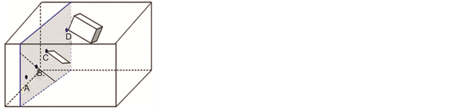
A prospecting line profile map is a virtual cutting plane to 3D geological model. The 3D point, curve and surface features on it are the downgrading dimension expression of 3D point, curve, surface and solid features in the 3D model. In most cases, a 3D point feature on 3D profile is a intersection point of 3D curve feature with the profile plane, as show in Figure 1(a)B; but in the extreme case, is a intersection of point, surface or solid feature with the profile plane, as show in Figure 1(a)A, Figure 1 (a)C and Figure 1(a)D. In most cases, a 3D curve feature on a 3D profile, is a intersection curve of 3D surface feature with the profile plane, as shown in Figure 1(b)B; but in the extreme cases, is a intersection of curve or solid feature with the profile plane, as shown in
 (a)
(a)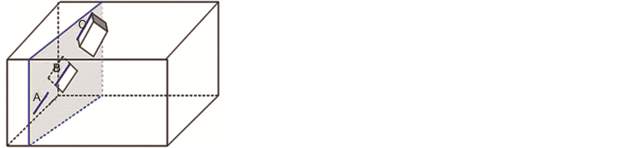 (b)
(b)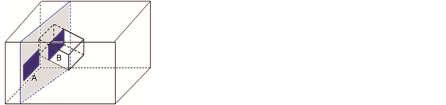 (c)
(c)
Figure 1. Representation of 3D point, curve, surface and solid features virtual cut by the prospecting line profile: (a) The intersection points of 3D point, curve, surface or solid feature with the prospecting line profile; (b) The intersection curve of 3D curve, surface or solid features with the prospecting line profile; (c) The intersection surface of 3D surface or solid features with the prospecting line profile.
Figure 1(b)A and Figure 1(b)C. In most cases, A 3D surface feature on 3D profile is a intersection of 3D solid feature with the profile plane as shown in Figure 1(c)A; but in the extreme case, is a intersection of surface feature with the profile plane, as shown in Figure 1(c)B.
By the view of geographic information science [9] [10] , the space dimension of geographic feature existed is number of coordinate components to describe a position in the space. Space dimension can be one, two, up to three dimension. The geology model is in a 3D space. The profile map paper space is a 2D space. Different from space dimension of features existed, dimension of a geographic feature is its extensible dimension. A point feature is a 0 dimension feature, because it cannot extend along any direction. A curve feature is a one dimension feature, because the feature can extend along one direction. A surface feature is a two dimension feature, because the feature can extend along two directions. Same argument, a solid feature is a three dimension feature. In a space, the dimension of feature must be lower or equal the dimension of the space. For example, in 3D space, could existed 0, 1, 2 and 3 D features. In 2D space, it only can exist 0, 1 and 2D feature, it cannot exist 3D feature. In the process of virtual cutting 3D geology model by prospecting line profile, the 3D solid features in the model downgrade to 2D polygon features in the 3D profile; 2D surface features downgrade to 1D curve feature; 1D curve feature downgrade to 0D point feature.
3. The Overall Shape and Conversion Process of Prospecting Line Profile
3.1. The Overall Shape of Prospecting Line Profile
Prospecting line profile is a figure created by virtual cutting geological model vertically along the prospecting line. Due to various reasons, drills on the prospecting line are not arranged in a straight line, it makes the prospecting line bent. The prospecting line profile thus becomes a composite surface of several conjoint vertical planes, which are horizontal bent along its strike line, the drilling positions are bending points. Figure 2(a) shows 3D spatial shape of the bending vertical profiles.
The prospecting line and prospecting line profile are bent in the 3D space, but drawing space of the profile map is 2D (paper), so the vertical surface which bends along exploration line was straightened after projecting onto 2D drawings space. This is a coordinate downgrading dimension process of from 3D space to 2D. Figure 2(b) shows the 2D spatial form of the bending vertical profiles.
The process of conversion from 3D profile to 2D profile, the coordinate dimension of features is downgrade from 3D to 2D. This paper doesn’t discuss this process. The process has been discussed by Wang [7] [8] .
3.2. Constructing 3D Prospecting Line Profile Frame
By extracting the 3D coordinates of the starting point, five drilling holes, and the end point of the prospecting line profile (the southwest start, 1 - 2, 1 - 17, 1 - 15, 1 - 1, shallow 1 - 1, the northeast end), building vertical section TIN and generating 3D prospecting line profile frame [11] . Schematic diagram shows in Figure 3(b).
 (a)
(a)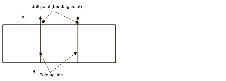 (b)
(b)
Figure 2. The 3D and 2D performance shape of bending vertical profiles: (a) 3D spatial shape of vertical profile; (b) 2D spatial shape of vertical profile.
3.3. Bending Section Subsection Conversion
Since the prospecting line profile is 2D, profile has only x, y coordinates. The y coordinates is usually associated with z coordinates of 3D space. The x coordinates of profile is associated with the x, y coordinates of 3D space. The y coordinate of the original geological profile points can be converted to z value of 3D space through reference of elevation line and scale of profile. The x coordinate of profile convert into the x, y value of 3D space by coordinate transformation. For the folded profile of changed direction, it needs to determine the trend of each folded cross-section (each section of folded angle exploration line and the X axis). Thus, the 3D coordinate (x, y, z) of each node on the fold profile can be calculated, and realize the conversion of 2D prospecting line profile to 3D.
Figure 3(a) is schematic of 2D prospecting line profile that virtual surface for the cutting of the geological model, where X′ and Y′ is the two vertical and horizontal coordinate axes of 2D prospecting line profile; Figure 3(b) is schematic of 3D prospecting line profile. Where “A” is the starting point of prospecting line profile, “B”, “C” and “D” presents three orifices of the drill points(turning point), their 2D coordinates of prospecting line profile and plane coordinates of 3D are known. “P” is a random point on fault line of prospecting line folded section A-B, its 2D coordinate is known in the prospecting line profile, θ1 is the angle between the AB side and the X axis, it is also the toward of the folded section; In the same way, the rest of the folded section direction is the angle corresponding exploration line with the X axis [12] .
In Figure 3(a), the A is a reference point, its
2D coordinates is (XA1, YA1) in the
profile, 2D coordinates of B point is (XB1, YB1),
marking the lowest point elevation is Zmin and the corresponding point
coordinate is Ymin, the 3D coordinates of A point and B point are (XA2,
YA2, ZA2) and (XB2,
YB2, ZB2), 2D coordinates of P point
is (XP1, YP1) in profile, the 3D coordinates
is (XB2, YB2, ZB2),
after conversion, the scale is .
.
Prospecting line AB and X axis angle
 expression is (1):
 (1)
(1)
The expression for the coordinate conversion is (2):
 (2)
(2)
3.4. Adding Switch Control Points
It can be seen in Figure 3(b), 3D prospecting line profile is not a simple flat profile but Zigzag section of varying
 (a)
(a) (b)
(b)
Figure 3. Illustration of the 2D and 3D profile: (a) 2D prospecting line profile; (b) 3D prospecting line profile.
direction. Converting two-dimensional coordinates of each line features of prospecting line profile directly will lead to partial line features out of the exploration profile. Result shows in Figure 4. A line which contains the E, F two nodes of the line features is not in the profile of prospecting line, so adding a turning control point G in the long edge of the turning point of the across profile is needed, then generate the E, G, F Folding line in the profile, so that the conversion curve falls on the bending profile.
3.5. The 3D Coordinates of Borehole Deviation Trajectory
During drilling, for the stratum conditions, drilling equipment, artificial operation and other reasons, boreholes are often deviation. After the borehole deviation, borehole trajectory becomes a 3D curve deviated from the the prospecting line profile. Therefore, the geological draftmen will calculate the 3D coordinates of the hole trace turning point according to zenith angle, azimuth angle and long of the borehole trace each subsection, then projected it to prospecting line profile. The drill trace turning points calculated by prospecting line profile after upgrading dimensional transformation inevitably fall in vertical plane located zigzag section, but it has some deviations from the reality. The more accurate practice to the drill trace should be read directly from the drill trace coordinate table.
3.6. Upgrading Feature Dimension from 1D Curve to 2D Surface
In 3D prospecting line profile, there are point, curve and polygon features. The second key of 3D geology modeling from 2D prospecting line profile is upgrading feature dimension from 1D curve to 2D surface. The curves of same geology surface (such as a coal seam floor surface or a fault surface) in different prospecting line profiles should be marked as same geo-surface id. Thus, the curves of one surface on adjacent profile could be as skeleton curves to make a surface. The process of make surface by skeleton curve is make irregular triangle net by the constrain curve in adjacent profiles, the method see work of Mallet [13] . The process is seen in Figure 9 and Figure 10. On the base of stratum interfaces and fault surfaces, it is easy to build stratum solid from these surfaces.
4. Experiments
4.1. Experimental Data
This experiment used thirteen prospecting line profile of a coal field in Chinese Qhinghai area as the original data. The prospecting line profile is opened as a MPJ project file in MapGIS (Including points, line, surface file), includes drilling opening and annotation, profile azimuth, orebody, lithology, grade, sampling number, strata, fault, drilling, name, picture frame, legend, responsibility table etc.

Figure 4. Illustration of adding turned control points.
In order to achieve the conversion from 2D exploration line profile to 3D exploration line profile, it needs to transform the line file of the prospecting line profile in. MPJ project file into standard graphic file DXF through MapGIS [14] , using G3DA (Geology Three dimensional Assistant Engineer) software to delete the graphic features which has little relationship with the reconstruction of three-dimensional geological model, only leaving features which is closely related to the reconstruction of 3D geological model, such as fault, stratigraphic boundary (coal seam floor), ground, bedrock top surface, drilling and elevation line, as shown in Figure 5.
Since 3D prospecting line profile is folded cross-sections of variable direction, in order to construct 3D prospecting line profile frame, It needs to regard the starting point, end point and the middle hole orifice points on the line of prospecting section as control points (the drill points between those starting point and ending point are the turning points of of the profile subsection). Extracting the plane coordinates (x, y) of control points in MapGIS as the x, y coordinates of the 3D space, extracting the coordinate x value of the corresponding points and elevation value z in the 2D prospecting line profile at the same time, z is regarded as z value of 3D space in it. In order to transform the geological factors of 2D prospecting line profile to 3D prospecting line profile, it needs to extract elevation Zmin of the lowest point that the profile marked and the corresponding Ymin, and regard them as initial data of 2D prospecting line profile node elevation values, and then write the path of file data of prospecting line profile in this area into the text file together.
The next is file data format: of prospecting line profile coordinate transform control (// follows note)
< file header="">
< file identification=""> profile coordinate transform control file
< planar map="" scale="" denominator="">5000
< profile line="" number="">1
< file body="">
< profile number="">1
< profile file name>F:\profile map\1line profile map.ds
< profile map="" scale="" denominator="">2000
< profile vertical="" scaling="" point=""> −93.62 3050
< the number="" of="" control="" points="">7 0
west south 974.25 936.61 −714.78 //control point name, x, y of plane map, x of profile
1-2 983.31 1093.85 −320.70
1-17 938.80 1193.27 −48.21
1-15 943.94 1249.92 93.56
1-1 948.85 1335.97 310.12
Shallow 1-1 949.77 1345.41 332.78
north east 953.55 1414.09 505.57

Figure 5. 2D prospecting line profile after processing.
4.2. Experimental Procedure
The authors use Microsoft visual studio 2010 development tools and C++/OpenGL in the “GE3DA” software platform. Firstly, by reading the 3D coordinates of turning points of the prospecting line profile, building vertical section TIN and generating 3D prospecting line profile frame, and then reading line file data of prospecting line profile in this area (2D coordinates of prospecting line profile), bending profiles are converted by section using method of 2D prospecting line map into 3D prospecting line map the proposed method in this paper and adding switch control points for the long line crossover two segments, realized the prospecting line profile from the data source to the layers hierarchical transformation.
4.3. Experimental Results
The 3D exploration line profile which is converted from the 2D exploration line profile shown as Figure 6. The original 2D profile is shown in Figure 5. It can be seen that the 3D profile after conversion maintained the geometry characters which the original 2D geological profile expressed. The thiteen adjacent 3D prospecting line profiles are shown in Figure 7. Three coal seam floor surfaces, which are constructed by seam floor contour map, are matched well with the thirteen 3D prospecting line profiles, as shown in Figure 8.
Figure 9 shows how to upgrade feature dimension from a 1D curve feature in 3D profile to 2D surface in 3D model, it is by triangulation between fault curves on adjacent 3D profiles. Figure 10 shows the fault surface in Figure 9 is smoothed by cubic spline surface method. The smooth method is seen in work of Sharma [15] and

Figure 6. 3D prospecting line profile after transformation.

Figure 7. Thriteen adjacent 3D prospecting line profile after transformation.

Figure 8. Thriteen 3D prospecting line profile and three coal seam floor surfaces, which are constructed by coal seam floor contour maps.

Figure 9. A fault surface is constructed by creating a TIN from constrain skeleton curves on adjacent 3D profiles.

Figure 10. The fault surface in Figure 9 is smoothed by cubic spline surface method [15] [16] .
Caliò [16] . Figure 11 shows the fault surfaces. Figure 12 shows the thirteen profiles and the three seam floor surfaces and the ten fault surfaces.
5. Conclusions
Construction 3D geological model from the prospecting line profile involves two times operation of upgrading dimension. The first upgrading dimension operation is upgrading points from 2D point in 2D profile into 3D points in 3D profile, i.e. from 2D profile into 3D profile. The second time upgrading dimensional operation is upgrading feature dimension from 3D point (0D), curve (1D) and surface (2D) feature on 3D profile into 3D curve (1D), surface (2D) and solid (3D) feature, in which the key is to construction surface form curves in the adjacent profiles.
Since the section of exploration line has the characteristics of direction changing zigzag section, a procedure of construction 3D model from 2D section map is proposed. It is 1) to construct 3D prospecting line profile

Figure 11. Ten fault surfaces constructed by fault curves in 3D profile and the thirteen 3D prospecting line profile.

Figure 12. Three coal seam floor surfaces, ten fault surfaces and thirteen 3D prospecting line profiles.
frame sectionalized, 2) transformation every point, curve and polygon in every profile section, 3) adding turning control point method in the long edge of the turning point of the cross section, and 4) construction surface from skeleton curves in adjacent 3D profile.
Through the experiment, it is realized that the various features of on the 2D prospecting line profile planed map ascend dimension transformed into 3D exploration line profile. The fault surface has been constructed from the fault curves in the 13 adjacent 3D profiles.
Acknowledgements
This work is supported by National Nature Science Foundation of China project “Theory and method of anisotropic property field inner geology body based on volume function” (Project number 41272367) and Open Foundation Project “Research on technical problems of 3D geological model data exchange format in the application of exploration and coal resources in digital mine” of Key Laboratory of Geological Information Technology, Ministry of Land and Resources (201407).
References
- Schumaker, L.L. (1990) Reconstructing 3D Objects from Cross-Sections. In: Dahmen, W., Gasca, M., Michelli, C., et al., Eds., Computation of Curves and Surfaces, Kluver Academic Publishers, Dordrecht, 275-309.
- Muller, H. and Klingert, A. (1993) Surface Interpolation from Cross Sections. In: Hagen, H., Muller, H. and Nielson, G.M., Eds., Focus on Scientific Visualization, Springer-Verlag, London, 139-189.
- Meyers, D. (1995) Reconstruction of Surfaces from Planar Contours. University of Washington, Seattle.
- Li, M.W., Zhao, C.S., Zheng, R.F., et al. (2005) A Study on Transformation Method Between the 3D Coordinates of a Geological Prospecting Line Section and the 2D Coordinates of the Line Section Drawing. Journal of Jilin University: Earth Science Edition, 3, 818-822.
- Li, G.Q., Chen, A.M., Deng, M. and Li, J.J. (2005) A New Transformation Method of Exploratory Profiles from 2D to 3D Coordination Systems. Modern Geology, 23, 2-3.
- Chen, J.H., Zhou, Z.Y., Chen, G. and Gu, D.S. (2005) Automatic Formation Method of Prospecting Line Profile Map Based on Drill Hole Database. Journal of Central South University (Natural Science), 36, 2-3.
- Wang, Z.G., Qu, H.G., Zhang, C.M. and Yao, L.Q. (2007) Triangulation Visualization of Three Dimensional Topological Geology Section. Geography and Geo-Information Science, 23, 1.
- Wang, Z.-G., Pan, M., Qu, H.-G., et al. (2008) Algorithm of Delaunay Triangulation of 3D Folded Cross-Section. Computer Engineering and Applications, 44, 94-96.
- ISO 19107 (2003) Geographic Information Spatial Schema. ISO TC 211.
- Herring, J. OGC Abstract Specifications Topic 1―Feature Geometry, 2001-05-10.
- Pilout, M., Tempfli, K. and Molenaar, M.A. (1994) Tetrahedron-Based 3D Vector Data Model for Geoinformation. Ad- vanced Geographic Data Modelling, 40, 129-140.
- Wang, D. (2009) Research on Three-Dimensional Geological Modeling Based on Planar Geological Map. Nanjing Normal University, Nanjing, 55-66.
- Mallet, J.-L. (2002) Geomodeling. Oxford University Press, Oxford.
- Liu, X. (2011) The Research on Key Algorithm of Three Dimensional Geological Modeling. University of Science and Technology of China, Hefei, 14-20.
- Sharma, J., Guha, R. and Sharma, R. (2011) Improved Ostrowski-Like Methods Based on Cubic Curve Interpolation. Applied Mathematics, 2, 816-823. http://dx.doi.org/10.4236/am.2011.27109
- Caliò, F. and Marchetti, E. (2013) Cubic Spline Approximation for Weakly Singular Integral Models. Applied Mathematics, 4, 1563-1567. http://dx.doi.org/10.4236/am.2013.411211