Open Journal of Earthquake Research
Vol.05 No.02(2016), Article ID:66906,8 pages
10.4236/ojer.2016.52009
The Stochastic Finite-Fault Modeling Based on a Dynamic Corner Frequency Simulating of Strong Ground Motion for Earthquake Scenario of North Tabriz Fault
Hadi Amiranlou1*, Mohsen Pourkermani1, Rouzbeh Dabiri2, Manoucher Qoreshi1, Soheila Bouzari1
1Department of Geology, Faculty of Basic Science, Islamic Azad University, North Tehran Branch, Tehran, Iran
2Department of Civil Engineering, Tabriz Branch, Islamic Azad University, Tabriz, Iran

Copyright © 2016 by authors and Scientific Research Publishing Inc.
This work is licensed under the Creative Commons Attribution International License (CC BY).
http://creativecommons.org/licenses/by/4.0/


Received 8 March 2016; accepted 27 May 2016; published 30 May 2016
ABSTRACT
The occurrence of the historical and machine Earthquakes, near to the North Tabriz Fault in NW Iran is an evidence for the seismic activity of this fault, which records a historical earthquake with a magnitude more than 7. Using the existing experimental relations, seismicity, and the fault geometry, a Mw 7.7 earthquake scenario was defined. The stochastic finite-fault modeling based on a dynamic corner frequency shows good agreement with common attenuation patterns. The shake map illustrates that Baghmisheh, Roshtieh, Ellahieh, Valiamr, and Eram region on Tabriz are at high hazard areas, and the maximum acceleration is located at the north direction with the same azimuth similar to fault strike.
Keywords:
Earthquake Scenario, Tabriz Fault, Tabriz, Shake Map

1. Introduction
The study area of Tabriz is selected in this work because the earthquake system record does not record any destructive event for Tabriz fault, and the estimation of strong ground motion predicts on the basis of the stochastic hypothetical model on this region. Simulating the earthquakes scenario is the best method for getting more knowledge on the earthquake event on Tabriz region. Therefore the simulating of strong ground motion was done at 252 points with 0.2 degree of distance at longitude and latitude in Tabriz region.
Strong ground motion is a physical complex process that includes three stages: earthquake waves are partial of strain energy released from fault, which is affiliated to source affect. Then the waves circulate the whole of earth crust, this phenomenon is called as route affect. And finally they are changed across shallow layers until they reach to the surface, which is called as site affect. This is illustrated in Figure 1.
The acceleration record machine creates variations in accelerogram that can be eliminated based on machine characteristic. Accelerogram is the result of these factors. The accelerogram characteristic is different for short and long period. Record of accelerogram at near the fault in Parkfield earthquake in 1966 provided scientific foundation for presenting a method for simulating of strong ground motion for the estimation of acclerogram time series. The methods are as: random (Boor, 1983); Empirical Greens Function (Hurtzel, 1978; Irikura, 1983; Hadely and Helembeger, 1980); Semi-Empirical Greens Function (Survanil, 1991; Midurakuva, 1993; Khatari, 1998; Hamzelu, 2000); composite source model (Khatari, 1995); hybrid (Kamae, 1998; Hamzelu, 2000). This method considers the information affiliated to source, route, site and attenuation in simulating of strong ground motion.
The stochastic method is used for the prediction of strong ground motion. This method is of two types: one is point source and the other is finite-fault method [1] [2] .
Point-source modelling of an earthquake reduces the entire fault plane into a single point, which is often taken as the location where the most energy is released. This is illustrated in Figure 2, where the fault surface is represented as a single point. Approximating an earthquake as a point greatly reduces the complexity of the source, as there is a reduced amount of geometry and no planar features. Although earthquake fault planes can be large, in the order of tens or hundreds of kilometers, this approximation holds well if the site is a large
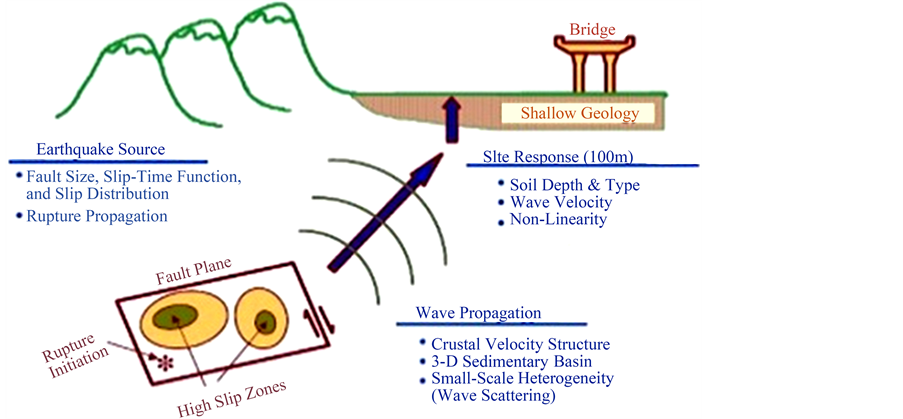
Figure 1. An illustration of the three physical processes that effect on the form of earthquake wave (Stuvart et al., 2001).

Figure 2. An illustration of point-source earthquake modelling. The fault plane is represented by a single point located on the fault.
distance away or the earthquake is small. The path length should be much larger than the fault length.
Finite-fault modelling uses the same process as point-source models; however, it breaks the fault plane into smaller subfaults. Each individual subfault acts as a separate point source; and the contribution of each subfault, along with an appropriate time delay, is summed to produce the larger desired effects. This type of modelling is illustrated in Figure 3. A finite-fault source is a bit more complex than a point source; however, the accuracy and time required for calculations increase as the total number of subfaults increases [2] .
The essence of this method is the target frequency spectrum of an earthquake, which is the most important determining factor of the resulting earthquake time series. A lot of research efforts (Boore, 1983; Atkinson and Boore, 1995; Haddon, 1996; Beresnev and Atkinson, 1998a; Motazedian and Atkinson, 2005) have been put into determining the best and simplest equations that describe the frequency content of an earthquake [1] [3] . The earthquake source parameters contain the parameters for the actual earthquake; the path effects describe the effects of the envelope propagating through a medium; and, the site effects contains the response of the location where the ground motions are felt.
2. Stochastic Finite-Fault Modelling
The earthquake fault plane is divided into N smaller subfaults, whose size can be anywhere from one kilometer to several kilometers in length and width. Each subfault is treated as a single earthquake, and a single time series is generated using a stochastic point-source technique. The final time series is calculated by summing the individual contributions of each subfault with the addition of an appropriate time delay:


Figure 3. An illustration of finite-fault modelling. The fault surface is divided into smaller fault segments, and each subfault is treated as a point source.
 (1)
(1)
where a(t) is the final time series, nl and nw are the total number of subfaults along the length and width, aij(t) is the time series for each ith and jth subfault, and Δtij is the time delay for the corresponding subfault.
The seismic moment for each subfault is determined from the ratio of the subfault to the main fault. If all the subfaults are identical, then:
 (2)
(2)
where M0ij is the seismic moment of a subfault.
If the subfaults are not identical, then the seismic moment can be determined from an array of slip weights, Sij, by:
 . (3)
. (3)
The summation of the slip weights array ensures that the sum of the subfault seismic moments is equal to the total seismic moment.
The acceleration spectrum for a subfault at a distance, Rij, can be modelled as a point source with an ω2 shape (Aki, 1967; Brune 1970; Boore, 1983). The acceleration of the ijth subfault,  , is described by (Motazedian and Atkinson, 2005):
 (4)
(4)
where f0ij is the subfault corner frequency.
 (5)
(5)
where is  the radiation pattern (average value is taken as 0.55 for shear waves), F is the free surface amplification (2.0), V is the partition onto two horizontal components (0.71), ρ is the density in kg/m3, and β is the shear wave velocity in km/s. EXSIM-V3 implements a dynamic corner frequency (Motazedian and Atkinson 2005), which has the corner frequency of a subfault change as the number of previously ruptured subfaults changes [4] . If NR(t) is the cumulative number of ruptured subfaults at time t.
 (6)
(6)
where f0ij(t) is the corner frequency of the ith, jth subfault at time t, and M0ave is the average seismic moment of the subfaults. Taking t = tend, then NR(tend) = N; and, the corner frequency becomes:
 . (7)
. (7)
This shows that the corner frequency at tend is the corner frequency of the entire fault (Motazedian and Atkinson, 2005). This dynamic corner frequency reduces the level of the spectrum and the radiated energy of each subfault at high frequencies, reducing the subfault size dependency.
In EXSIM_V3, a scaling factor, Hij, is used to conserve the total radiated energy of high frequencies for the subfaults [4] . The acceleration spectrum with this scaling factor is:
 . (8)
. (8)
Requiring conservation of energy between the energy radiated from a subfault with the scaling factor and the average energy radiated from a subfault (Motazedian and Atkinson 2005; Boore, 2009), the scaling factor is:
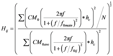 (9)
(9)
where hc is the high-frequency filter.
3. Research Method
The statistic research shows the last damaging earthquake on Tabriz region occurred in 1819 [5] [6] . The earthquake system record does not record any destructive event for Tabriz fault. The estimation of strong ground motion predicts on the basis of the stochastic hypothetical model on this region, and simulating the earthquakes scenario is the best method for getting more knowledge on the earthquake event. Therefore earthquake scenario was defined based on Tabriz fault geometry, destructive historical earthquake and seismology history. Based on existing experimental equation and seismicity obtain the ability of creation earthquake with Mw more than 7.5 and 60 km rupture length for Tabriz fault [7] .
For simulating Tabriz north fault scenario earthquake was used stochastic finite-fault method based on dynamic corner frequency [2] . Finite-fault modeling uses the same process as point-source models, however it breaks the fault plane into smaller sub fault. Each sub fault acts as a separate point source; and the contribution of each sub fault along, with an appropriate time delay, is summed to produce the larger desired effects [2] . In stochastic finite-fault modeling, corner frequency is functional based on time and frequency content of simulating time series at sub fault was controlled by rupture history [2] . Rupture begins with an extra corner frequency and it reduces with growth of rupture plane [2] . Geometry of fault was determined based on geology information, seismology and existent equation [5] [7] - [9] . It has been mentioned in Table 1.
Earthquake parameters were used such as geometrical spreading, quality factor and stress drop obtained from research that has been done for north of Iran earthquakes [2] [10] - [13] . It has been mentioned in Table 2.

Table 1. Tabriz north fault geometry.
Table 2. Parameters was used for simulating.
The place of hypocenter was located at the nearest distance to city. Depth of fault was selected based on the average depth obtained from research.
The simulating was performed based on the mentioned parameters on the seismicity bed rock surface. A sample of simulating accelerogram is illustrated in Figure 4. With the extraction of maximum acceleration and the drawing of them based on distance show a good coordination with the general attenuation type [10] [14] - [17] . It is illustrated in Figure 5. The shake map was drawn with use of the maximum acceleration on the seismicity bed rock surface at netting point on Tabriz region. It is illustrated in Figure 6.
4. Conclusions
1) With use of the existing experimental equation and seismicity, the ability of creation earthquake with Mw more than 7.5 and 60 km rupture length for Tabriz fault was obtained. Therefore earthquake scenario was defined as Mw 7.7 for Tabriz fault.
2) The simulating was performed based on the mentioned parameters on the seismicity bed rock surface. With

Figure 4. An illustration of a type of simulating accelerogram.

Figure 5. Illustrate strong ground motion based on distance.

Figure 6. Illustrate shake map (PGA).
the extraction of maximum acceleration and the drawing of them based on distance, a good coordination with the general attenuation type was shown, especially with (Hamzehloo et al., 2015) attenuation pattern for NW Iran.
3) The shake map illustrates that Baghmisheh, Roshtieh, Ellahieh, Valiamr, and Eram region on Tabriz are at high hazardous areas, and the maximum acceleration is located at the north direction with the same azimuth similar to fault strike.
Cite this paper
Hadi Amiranlou,Mohsen Pourkermani,Rouzbeh Dabiri,Manoucher Qoreshi,Soheila Bouzari, (2016) The Stochastic Finite-Fault Modeling Based on a Dynamic Corner Frequency Simulating of Strong Ground Motion for Earthquake Scenario of North Tabriz Fault. Open Journal of Earthquake Research,05,114-121. doi: 10.4236/ojer.2016.52009
References
- 1. Boore, D.M. (2003) Simulation of Ground Motion Using the Stochastic Method. Pure and Applied Geophysics, 160, 635-676. http://dx.doi.org/10.1007/PL00012553
- 2. Motazedian, D. and Atkinson, G.M. (2005) Stochastic Finite-Fault Modeling Based on a Dynamic Corner Frequency. Bulletin of the Seismological Society of America, 95, 995-1010. http://dx.doi.org/10.1785/0120030207
- 3. Beresnev, I. and Atkinson, G. (2002) Source Parameters of Earthquakes in Eastern and Western North America Based on Finite-Fault Modeling. Bulletin of the Seismological Society of America, 92, 695-710.
- 4. Stephen, C. and Motazedian, D. (2011) A Guide for Using EXSIM-V3 a Stochastic Finite-Fault Modelling Technique with Low-Frequency Scaling.
- 5. Ambraseys, N.N. and Melville, C.P. (1982) A history of Persian Earthquakes. Cambridge University Press, UK, 219.
- 6. Berberian, M. (1994) Natural Hazards and the First Earthquake Catalogue of Iran. Vol. 1: Historical Hazards in Iran Prior to 1900. A UNESCO/IIEES Publication during UN/IDNDR: International Institute of Earthquake Engineering and Seismology, Tehran, Iran.
- 7. Wells, D.L. and Coppersmith, K.J. (1994) New Empirical Relationships among Magnitude, Rupture Length, Rupture width, Rupture Area and Surface Displacement. Bulletin of the Seismological Society of America, 84, 974-1002.
- 8. Hamzelu, H., Farzanegan, A. and Alavicheh, H. (1389) Mechnism of Tabriz Earthquake in 10 Azar with Use of Acceleration Data. Journal of Geology Science, No. 75.
- 9. Siahkali Moradi, A., Hatsfeld, D. and Pal, A. (1387) Research Crust Velocity Structure and Mechanism Faulting in Tabriz Strike Slip Region. Journal of Geology Science, No. 70.
- 10. Akbarzadeh, N., Mahood, M. and Hamzehloo, H. (2012) Attenuation Relationship for the Horizontal Component of Peak Ground Acceleration and Acceleration Response Spectra in NW Iran. Geophisice Magazine of Iran, 6, No. 1.
- 11. Boore, D.M., Campbell, K.W. and Atkinson, G.M. (2010) Determination of Stress Parameters for Eight Well-Recorded Earthquakes in Eastern North America. Bulletin of the Seismological Society of America, 100, 1632-1645. http://dx.doi.org/10.1785/0120090328
- 12. Nezanaslami, H. (1382) Determination of Quality Factor for Tabriz Region. M.sc. Thesis, Geophysical Institute of Tehran University.
- 13. Sharifi, M., Bairamnrjad, A. and Shomali, Z.H. (1391) Determination of Empirical Attenuation Coefficient for West North of Iran Based on Accelerogram. 15th Iran Geophisic Conferences, Iran, 15-17 May 2012, 96-100.
- 14. Akkar, S. and Bommer, J.J. (2009) Empirical Equations for the Prediction of PGA, PGV and Spectral Accelerations in Europe, the Mediterranean Region and the Middle East. Seismological Research Letters, 81, 195-206.
- 15. Alahyarkhani, M. (2003) Attenuation and Propagation characteristics of Seismic Waves in Iran. Fourth International Conference of Earthquake Engineering and Seismology, Iran, 11-13 May 2003, 797-804.
- 16. Hamzehloo, H. and Mahood, M. (2012) Ground-Motion Attenuation Relationship for East Central Iran. Bulletin of the Seismological Society of America, 102, 2677-2684.
- 17. Hamzehloo, H., Mahood, M. and Akbarzadeh, N. (2015) Ground-Motion Amplitudes for Earthquakes in NW Iran. 7th International Conference of the Seismology and Earthquake Engineering, Iran, 18-21 May 2015, 1-6.
NOTES

*Corresponding author.