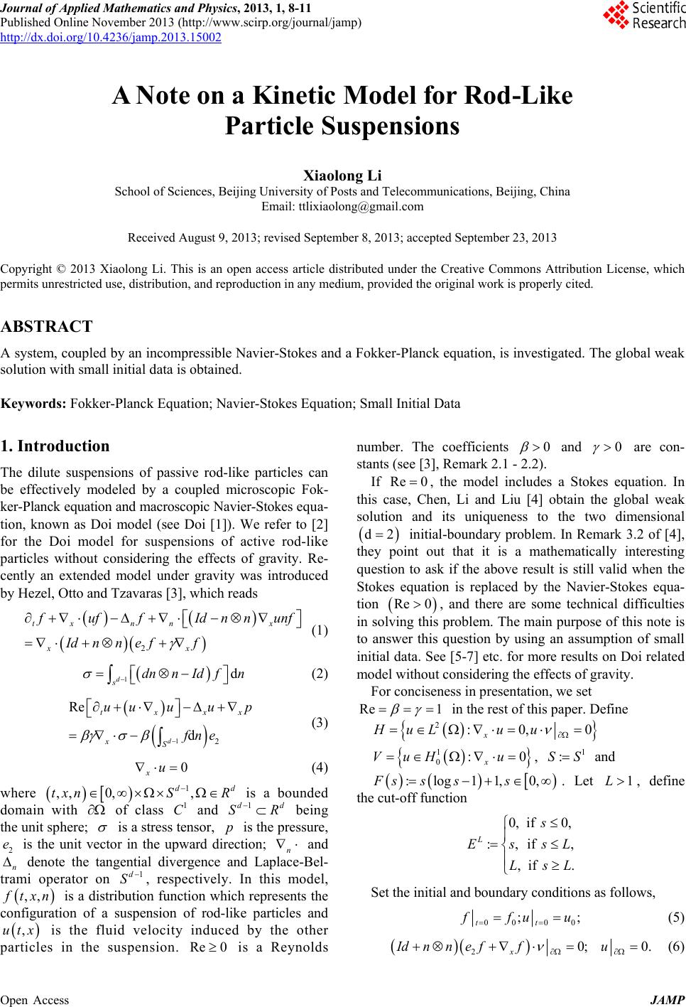
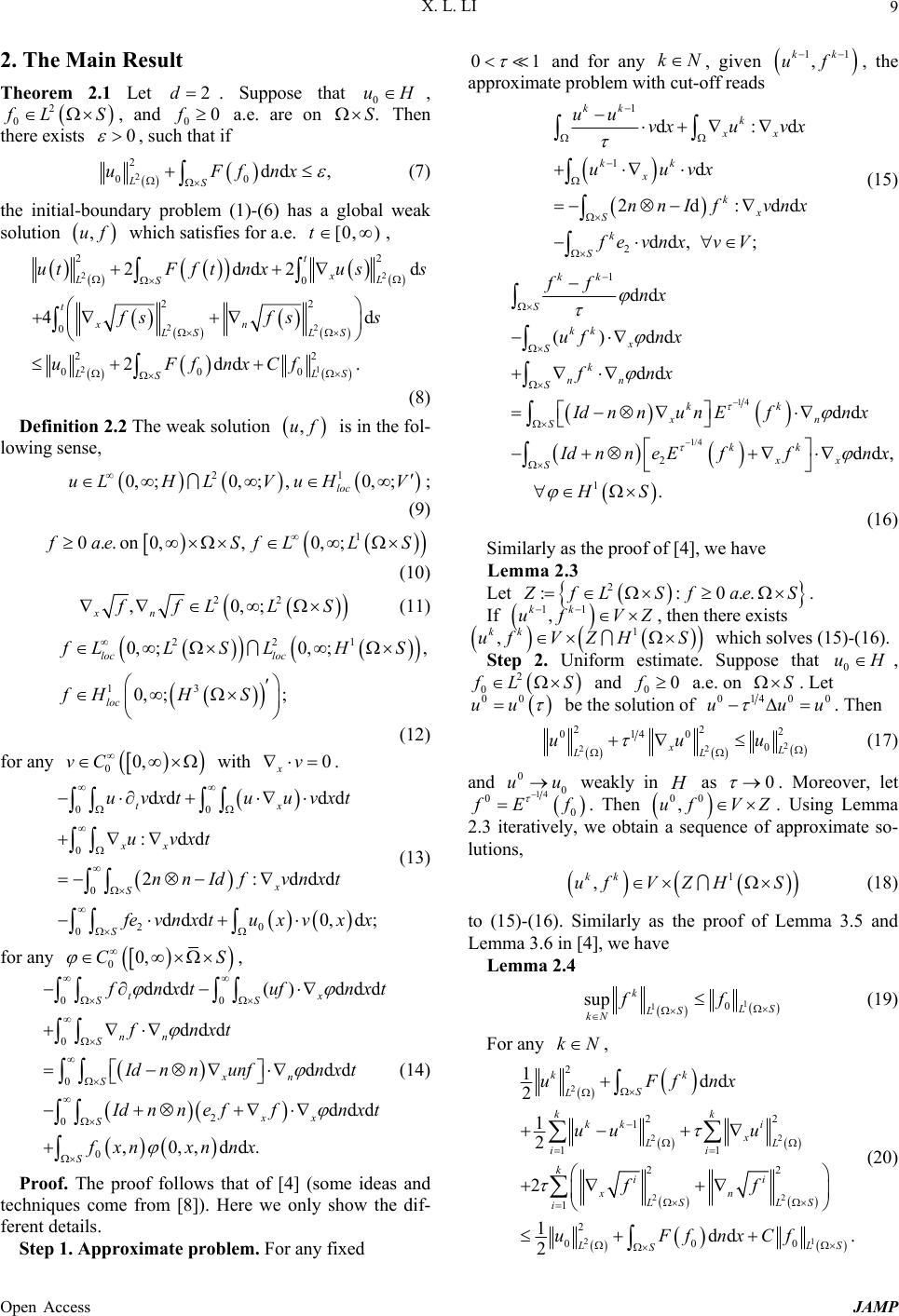
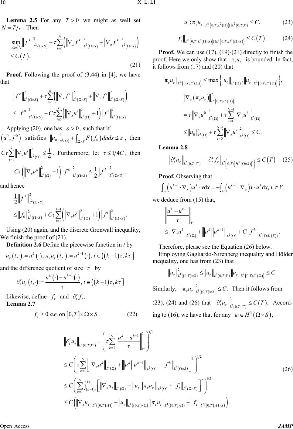
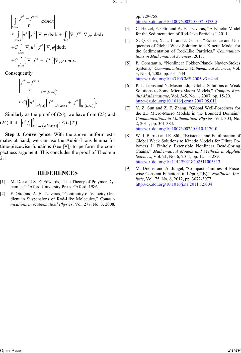
 Journal of Applied Mathematics and Physics, 2013, 1, 8-11 Published Online November 2013 (http://www.scirp.org/journal/jamp) http://dx.doi.org/10.4236/jamp.2013.15002 Open Access JAMP A Note on a Kinetic Model for Rod-Like Particle Suspensions Xiaolong Li School of Sciences, Beijing University of Posts and Telecommunications, Beijing, China Email: ttlixiaolong@gmail.com Received August 9, 2013; revised September 8, 2013; accepted September 23, 2013 Copyright © 2013 Xiaolong Li. This is an open access article distributed under the Creative Commons Attribution License, which permits unrestricted use, distribution, and reproduction in any medium, provided the original work is properly cited. ABSTRACT A system, coupled by an incompressible Navier-Stokes and a Fokker-Planck equation, is investigated. The global weak solution with small initial data is obtained. Keywords: Fokker-Planck Equation; Navier-Stokes Equation; Small Initial Data 1. Introduction The dilute suspensions of passive rod-like particles can be effectively modeled by a coupled microscopic Fok- ker-Planck equation and macroscopic Navier-Stokes equa- tion, known as Doi model (see Doi [1]). We refer to [2] for the Doi model for suspensions of active rod-like particles without considering the effects of gravity. Re- cently an extended model under gravity was introduced by Hezel, Otto and Tzavaras [3], which reads 2 tx nnx xx uffId nnunf Idnne ff (1) 1d d sdnnId fn (2) 12 Re d d txx xS uu uu p fne x d d R (3) 0 xu (4) where is a bounded domain with of class and being the unit sphere; 1 ,, 0,, d txnS R 1 C1d S is a stress tensor, is the pressure, is the unit vector in the upward direction; n p 2 e and n denote the tangential divergence and Laplace-Bel- trami operator on , respectively. In this model, 1d S ,, tx x n Re 0 is a distribution function which represents the configuration of a suspension of rod-like particles and is the fluid velocity induced by the other particles in the suspension. is a Reynolds ,ut number. The coefficients 0 and 0 are con- stants (see [3], Remark 2.1 - 2.2). If Re 0 , the model includes a Stokes equation. In this case, Chen, Li and Liu [4] obtain the global weak solution and its uniqueness to the two dimensional 2d initial-boundary problem. In Remark 3.2 of [4], they point out that it is a mathematically interesting question to ask if the above result is still valid when the Stokes equation is replaced by the Navier-Stokes equa- tion Re 0, and there are some technical difficulties in solving this problem. The main purpose of this note is to answer this question by using an assumption of small initial data. See [5-7] etc. for more results on Doi related model without considering the effects of gravity. For conciseness in presentation, we set Re 1 in the rest of this paper. Define 2:0, x HuLu u 0 1 0:0 x VuHu , and 1 :SS :log11, 0,Fs sss . Let , define the cut-off function 1L 0, if0, :,if ,if. L s Ess LsL ,L Set the initial and boundary conditions as follows, 00 00 ; tt ; fu u (5) 20; 0. x Idnneffu (6)  X. L. LI 9 2. The Main Result Theorem 2.1 Let . Suppose that 2d0 uH , 2 0 LS, and 0 a.e. are on Then there exists 0f.S 0 , such that if 2 2 00 dd , LS uFfnx (7) the initial-boundary problem (1)-(6) has a global weak solution which satisfies for a.e. , ,uf [0, )t 22 22 21 22 t 0 22 0 22 000 2dd2 d 4d 2dd . x LL S t xn LS LS LLS S utFf tnxuss fsfs s uFfnxCf (8) Definition 2.2 The weak solution is in the fol- lowing sense, ,uf 21 0,;0,; ,0,; loc uLH LVuHV ; (9) 1 0..on0,, 0,; aeS fLLS (10) 22 ,0,; xn fLL S (11) 221 13 0, ;0, ;, 0, ;; loc loc loc LLSLHS fHH S (12) for any with . 00,vC 0 xv 00 0 0 20 0 dd dd :dd 2:ddd ddd0, d; tx xx x S S uvxtuu vxt uvxt nnIdf vnxt evnxtuxv xx (13) for any 00,CS , 00 0 0 2 0 0 ddd( )ddd ddd ddd ddd ,0,,dd. tx SS nn S xn S xx S S nxtuf nxt fnxt Idnnunfn x t dnnef fnxt fxn xnnx (14) Proof. The proof follows that of [4] (some ideas and techniques come from [8]). Here we only show the dif- ferent details. Step 1. Approximate problem. For any fixed 01 and for any kN , given 11 , kk uf , the approximate problem with cut-off reads 1 1 2 d: d 2d:d dd, ; kk k xx kk x kx S k S uu vxu vx uuvx nnIf vnx fe vnxv V d d (15) 14 1/4 1 2 1 dd ()dd dd dd dd, . kk S kk x S k nn S kk xn S kk xx S ff nx uf nx fnx IdnnunEfn x dnneE ffnx HS (16) Similarly as the proof of [4], we have Lemma 2.3 Let 2 ::0.. fLSf ae S . If 11 , kk uf VZ , then there exists ,S 1kk ufV ZH which solves (15)-(16). Step 2. Uniform estimate. Suppose that 0 uH , 2 0 fL S and a.e. on . Let 00fS 00 uu be the solution of 0140 0 uuu . Then 2 22 22 2 0140 0xL LL uuu (17) and weakly in as 0 0 uuH0 . Moreover, let 14 0 0 fEf . Then 00 ,uf VZ . Using Lemma 2.3 iteratively, we obtain a sequence of approximate so- lutions, 1 , kk ufV ZHS (18) to (15)-(16). Similarly as the proof of Lemma 3.5 and Lemma 3.6 in [4], we have Lemma 2.4 1 10 sup k S LS kN ff (19) For any kN , 2 22 22 21 2 22 1 11 22 1 2 000 1dd 2 1 2 2 1dd . 2 kk S L kk kk i x LL ii kii xn LS LS i LS S uFfnx uu u ff uFfnxCf (20) Open Access JAMP  X. L. LI Open Access JAMP 10 Lemma 2.5 For any we might as well set 0T NT . Then 22 0, ;0, ; ;π. LTL LTV uu C (23) 22 22 11 sup . N kkk xn LSLS LS kN k fff CT 221 0, ;0, ;. LTL SLTH S fC T (24) 2 2 (21) Proof. We can use (17), (19)-(21) directly to finish the proof. Here we only show that πu is bounded. In fact, it follows from (17) and (20) that Proof. Following the proof of (3.44) in [4], we have that 22 22 22 1 22 0 1 1. k ki xn LSLS LS i kii x 22 0 0, ;0, ; πmax ,, LTLL LTL uuu 2 2 2 2 2 i SL i fff fCu f 22 22 22 2 0, ; 1 22 0 1 12 2 0 0 π . xLTL Ni xx LL i Ni x LL i u uu uu C LS Applying (20), one has 0 , such that if 00 ,uf satisfies 2 2 00 LS uFfdndx , then 2 2 1 1 4 ki xL i Cu Lemma 2.8 . Furthermore, let 14C , then 222 22 2 1 1, 2 kk k xLLSL Cu ff 223 0, ;0, ; tt LTVLTH S uf CT (25) S Proof. Observing that 11 dd kkk k xx uuvxuvuxv and hence ,V 2 222 2 122 2 0 1 1 2 1. k LS kii x LS LS i f fCu f we deduce from (15) that, 22 2 1 1 :. kk V kkk k xLL L uu uuu Cf 1 LS Using (20) again, and the discrete Gronwall inequality, We finish the proof of (21). Definition 2.6 Define the piecewise function in t by Therefore, please see the Equation (26) below. 1 ,: , ,:,1, kk ut uut utkk Employing Gagliardo-Nirenberg inequality and Hölder inequality, one has from (23) that and the difference quotient of size by 42 2 2 0,0, ;0, ;. LTLTV LTL uuu C 1 ,:, 1, kk t uu utt kk Similarly, 4 2 0, π. LT u C Then it follows from Likewise, define and . t (23), (24) and (26) that 2 2 0, ;. tLTV uC T Accord- Lemma 2.7 0..on0, . ae TS ing to (16), we have that for any 3 S , (22) 2 22 2 22 2 24 42 12 2 1 0, ;1 12 2 1 1 12 2 1 1 0,0,0,0, . kk N tLTV kV Nkkk k xLLS L k Nk xLLS L k k xLTLTLTLTS uu u Cuuu f Cuuuf Cu uuf (26)  X. L. LI 11 1 dd dd dd dd dd. kk S kk k xnn SS kk xn S kk xx S ff nx uf nxf nx Cuf nx Cff nx Consequently 3 12 1 1 . kk HS kk k HLSH ff Cu ff S Similarly as the proof of (26), we have from (23) and (24) that 23 2 0, ;. tLTH S CT Step 3. Convergence. With the above uniform esti- mates at hand, we can use the Aubin-Lions lemma for time-piecewise functions (see [9]) to perform the com- pactness argument. This concludes the proof of Theorem 2.1. REFERENCES [1] M. Doi and S. F. Edwards, “The Theory of Polymer Dy- namics,” Oxford University Press, Oxford, 1986. [2] F. Otto and A. E. Tzavaras, “Continuity of Velocity Gra- dient in Suspensions of Rod-Like Molecules,” Commu- nications in Mathematical Physics, Vol. 277, No. 3, 2008, pp. 729-758. http://dx.doi.org/10.1007/s00220-007-0373-5 [3] C. Helzel, F. Otto and A. E. Tzavaras, “A Kinetic Model for the Sedimentation of Rod-Like Particles,” 2011. [4] X. Q. Chen, X. L. Li and J.-G. Liu, “Existence and Uni- queness of Global Weak Solution to a Kinetic Model for the Sedimentation of Rod-Like Particles,” Communica- tions in Mathematical Sciences, 2013. [5] P. Constantin, “Nonlinear Fokker-Planck Navier-Stokes Systems,” Communications in Mathematical Sciences, Vol. 3, No. 4, 2005, pp. 531-544. http://dx.doi.org/10.4310/CMS.2005.v3.n4.a4 [6] P. L. Lions and N. Masmoudi, “Global Solutions of Weak Solutions to Some Micro-Macro Models,” Comptes Ren- dus Mathematique, Vol. 345, No. 1, 2007, pp. 15-20. http://dx.doi.org/10.1016/j.crma.2007.05.011 [7] Y. Z. Sun and Z. F. Zhang, “Global Well-Posedness for the 2D Micro-Macro Models in the Bounded Domain,” Communications in Mathematical Physics, Vol. 303, No. 2, 2011, pp. 361-383. http://dx.doi.org/10.1007/s00220-010-1170-0 [8] W. J. Barrett and E. Süli, “Existence and Equilibration of Global Weak Solutions to Kinetic Models for Dilute Po- lymers I: Finitely Extensible Nonlinear Bead-Spring Chains,” Mathematical Models and Methods in Applied Sciences, Vol. 21, No. 6, 2011, pp. 1211-1289. http://dx.doi.org/10.1142/S0218202511005313 [9] M. Dreher and A. Jüngel, “Compact Families of Piece- wise Constant Funcitons in L^p(0,T;B),” Nonlinear Ana- lysis, Vol. 75, No. 6, 2012, pp. 3072-3077. http://dx.doi.org/10.1016/j.na.2011.12.004 Open Access JAMP
|