Wireless Sensor Network
Vol. 4 No. 11 (2012) , Article ID: 24870 , 8 pages DOI:10.4236/wsn.2012.411039
SCHS: Smart Cluster Head Selection Scheme for Clustering Algorithms in Wireless Sensor Networks
1Electronics and Communication Engineering Department, Malaviya National Institute of Technology, Jaipur, India
2Computer Engineering Department, Malaviya National Institute of Technology, Jaipur, India
3Vice-Chancellor, Rajasthan Technical University, Kota, India
Email: vipinrwr@yahoo.com, girdharisingh@rediffmail.com, rp_yadav@yahoo.com
Received September 29, 2012; revised October 27, 2012; accepted November 4, 2012
Keywords: Wireless Sensor Network; Clustering; Energy Efficiency; Intra-Cluster Communication
ABSTRACT
Wireless sensor networks are energy constraint networks. Energy efficiency, to prolong the network for a longer time is critical issue for wireless sensor network protocols. Clustering protocols are energy efficient approaches to extend the lifetime of network. Intra-cluster communication is the main driving factor for energy efficiency of clustering protocols. Intra-cluster energy consumption depends upon the position of cluster head in the cluster. Wrongly positioned clusters head make cluster more energy consuming. In this paper, a simple and efficient cluster head selection scheme is proposed, named Smart Cluster Head Selection (SCHS). It can be implemented with any distributed clustering approach. In SCHS, the area is divided into two parts: border area and inner area. Only inner area nodes are eligible for cluster head role. SCHS reduces the intra-cluster communication distance hence improves the energy efficiency of cluster. The simulation results show that SCHS has significant improvement over LEACH in terms of lifetime of network and data units gathered at base station.
1. Introduction
Recently many researchers have shown great interest in wireless sensor networks [1] due to their wide range of application in the field of military surveillance [2], fire detection [3], habitat monitoring [4], industry [5], health monitoring [6] and many more. Wireless sensor networks [1,7] are composed of large number of randomly deployed sensor nodes. Sensor nodes are deployed within concerned area or very next to it. Wireless sensor net-works have at least one base station that works as a gateway between the sensor network and outside world. Sensor nodes sense the phenomenon and send the data to base station via single or multi-hop communication. Users access the data stored at base station.
Sensor nodes have limited battery power, memory and processing capabilities. So lifetime of a wireless sensor network is limited by on-board energy of sensor nodes. Due to harsh deployed area, replacement or recharge of battery is not feasible. Lack of infrastructure and large number of sensor nodes causes huge flow of message transfer through the network. As most of the energy is consumed during communication [7], currently different clustering algorithms [8,9] are proposed for wireless sensor networks to use energy of nodes efficiently.
Clustering algorithms are used in wireless sensor networks to reduce energy consumption. Operation of clustering algorithm is executed in rounds and each round is composed of two phases: setup phase and steady phase. Nodes are organized in independent sets or clusters. At least one cluster head is selected for each cluster. The sensed data is not directly sent to the base station but via respective cluster heads. Cluster head collects data of sensor nodes that belongs to that cluster. Clustering algorithms apply data aggregation techniques [8,16] which reduce the collected data at cluster head in the form of significant information. Cluster heads then send the aggregated data to base station.
Cluster head selection plays significant role for energy efficiency of clustering algorithms. Intra-cluster communication distance depends upon position of selected cluster head in a cluster and intra-cluster energy consumption depends upon intra-cluster communication distance. Clusters with high intra-cluster communication distance will consume more energy than other clusters. In this paper, a simple and efficient smart cluster head selection (SCHS) scheme is proposed that reduces the intra-cluster communication distance. The simulation results show that SCHS has significant improvement over LEACH [10] in terms of lifetime of network and data units gathered at base station.
The rest of paper is organized as follows. Section 2 describes the clustering schemes proposed in literature. Section 3 details network model and Section 4 discusses the significance of intra-cluster communication and the proposed solution to reduce it. Simulation results are shown in Section 5. Section 6 concludes the paper and scope of future work.
2. Related Review
LEACH (Low Energy Adaptive Cluster Hierarchy) [10] is fully distributed algorithm. In set-up phase cluster heads selection, cluster formation and TDMA scheduling are performed. In steady phase, nodes send data to cluster head and cluster head aggregate the data. Aggregated data is send to base station. After a fix round time, reclustering is performed. Role of cluster head is rotated to all the sensor nodes to make the network load balance. LEACH scheme does not guarantee about equal number of cluster heads in each round.
EBUC (Energy-Balanced Unequal Clustering) [11] is a centralized protocol that organize network in unequal clusters and CHs relay data of other CHs via multi-hop routing. PSO is applied at BS to select high energy nodes for CH role and for formation of clusters with unequal nodes. Clusters closer to BS are formed of small size to consume less intra-cluster energy and hence are ready for inter-cluster communication energy consumption. But protocol works only when BS is located outside the interested working area.
ADRP (Adaptive Decentralized Re-clustering Protocol) [12] selects a cluster head and set of next heads for upcoming few rounds based on residual energy of each nodes and average energy of cluster. In the initial phase, nodes send status of their energy and location to base station. Base station partitions the network in clusters and selects a cluster head for each cluster along with a set of next heads. In the cycle phase, cluster head aggregates the data and sends to the base station. In the re-cluster stage, nodes transit to cluster head from set of next heads without any assistance from base station. If the set of next heads is empty, initial phase is executed again.
EAP (Energy-Aware Routing Protocol) [17] provides new parameters for cluster head selection to handle heterogeneous energy of nodes. A node maintains a table of residual energy of neighbouring nodes within cluster range of node to calculate average residual energy of all these nodes. A node having residual energy higher than average residual energy has high probability of cluster head selection.
DEEC (Distributed Energy-Efficient Clustering) [13] has a two-level heterogeneous network. Sensor nodes are categorized in two types: advance nodes and normal nodes. Advanced nodes have higher energy than normal nodes. Initial and residual energy level of nodes is used for cluster head selection. So the high energy nodes are more probabilistic to select as cluster head than low energy nodes. High energy nodes are doing more work while low energy level nodes are doing work of sensing. EEHC (Energy Efficient Heterogeneous Clustering) [14] extended the node heterogeneity to three types: super nodes, advance nodes and normal nodes.
None of the schemes have a view on cluster head selection such that to minimize intra-cluster communication. Work of this paper proposed a simple and efficient cluster head selection scheme that reduce intra-cluster communication and extend lifetime of network.
3. Network Model
In our proposed protocol following network assumptions are considered:
• All sensor nodes are homogenous.
• All nodes are stationary once deployed in the field.
• Nodes are location aware i.e. nodes are equipped with any GPS device or use some method to find location.
• There is single base station located outside the field.
• All nodes have data to send.
• The nodes are considered to die only when their energy is exhausted.
3.1. Energy Model
In Wireless sensor networks, nodes are deployed randomly, i.e. positions of nodes are not pre-engineered. Most of the energy is dissipated during communication in sensor networks as it depends on the distance between the two nodes. Energy dissipation model is shown in Figure 1.
Both sending and receiving process of data communication consumes energy. According to energy model proposed in [7], for sending m-bit data over a distance d, the total energy consumed by a node is given by:
 (1)
(1)
and hence
 (2)
(2)
while the energy consumption for receiving that message is given by:
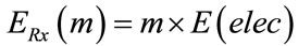 (3)
(3)

Figure 1. Radio energy dissipation model.
4. Problem Statement and Proposed Solution
4.1. Problem Statement
4.1.1. Intra-Cluster Distance
Intra-cluster distance and total cluster distance are synonyms. Total cluster distance is the measure of intracluster communication. Total cluster distance is defined as the sum of the distance of all nodes in the cluster to cluster head as in Equation (4).
 (4)
(4)
where N is the number of nodes in a cluster and Distance (i,CH) is distance of a node to cluster head. Energy efficiency of a cluster depends on the intra-cluster communication. The steady phase of clustering approach is longer than the set-up phase. In steady phase there is intra-cluster communication between nodes to cluster head and long distance inter-cluster communication between cluster heads and base station. Intra-cluster communication phase involves all sensor nodes and hence communication is much higher than inter-cluster communication. So intra-cluster communication consumes most of the energy from the network. Hence clusters with less total cluster distance are considered as more energy efficient.
4.1.2. Effect of Cluster Head Selection on Intra-Cluster Distance
Figure 2 shows a network with 50 nodes deployed randomly and uniformly over a 50 × 50 m2 area. The network is considered having a single cluster. The total cluster distance is calculated for each node considering it as cluster head.
Table 1 shows that clusters having cluster head nodes positioned near the center of cluster have less total cluster distance, while cluster head nodes positioned far from the center of cluster have large total cluster distance. So cluster head selection is an important issue and it affects energy efficiency of clustering approach drastically incase of improper selection. Hence the cluster head selection should be optimized to minimize intra-cluster communication.

Figure 2. Sensor network deployment with 50 nodes over 50 × 50 m2.

Table 1. Total intra-cluster distance of nodes.
4.2. Solution Statement
Various approaches are proposed for cluster formation and cluster head selection optimization for energy efficient communication. But most of the schemes cannot be implemented with distributed clustering algorithms because these schemes involve complex and intelligent computing. Sensor nodes have low storage circuitry and the computing is extremely energy consuming. So a new and simple to implement approach is required for cluster formation optimization for distributed approaches. The work of this paper proposes a fairly simple and easy to implement distributed scheme to optimize cluster head selection. As discussed earlier, cluster head selection is important for any cluster to be energy efficient.
Sensor nodes are deployed randomly in the field, i.e. there is no pre-engineered node deployment. Nodes can have their location by means of some localization algorithm or the nodes are equipped with some device, like GPS, that finds their exact location in the field, i.e. all the nodes know about their field location. In a distributed approach with dynamic clusters, clusters are formed in each round, i.e. there are no fix boundaries for clusters. In our proposed scheme, the total field area is divided into two parts: border area and inner area as shown in Figure 3. Division of area is an important issue for SCHS. Let d is the distance for partitioning of field. Area starting from boundary of the field up to the distance d is border area and the remaining inside area is inner area. The border area nodes do not participate in cluster head selection. Only the inner area nodes participate in cluster head selection. The border area nodes are always member nodes in each round. As the cluster head is always selected from the inner area in our scheme, therefore the cluster head is always close to center of the cluster. As discussed earlier, such clusters have less intra-cluster communication distance and hence more energy efficient.
Value of d for partitioning network is very crucial. A higher value for d makes inner area very small therefore there are few nodes for cluster head role that consume their energy very quickly. Hence network sustain for

Figure 3. Division of network area.
short time. While a lower value for d does not have enough change in network. Value of d for partitioning the network is analyzed in Section 5.2.
Cluster head nodes consume more energy than other nodes. In proposed scheme, though inner area nodes attempt a number of times for cluster head, but still network is load balanced and sustain for long time. Because inner area nodes has to communicate for short distance as cluster head is also from inner area. And border area nodes have always long communication distance as compared to other nodes but never attempt for cluster head role.
4.2.1. SCHS with Distributed Clustering Algorithm
Figure 4 shows the block diagram of the proposed SCHS with distributed clustering. In the set-up phase, each node is checked whether it belongs to border area or to inner area. If a node belongs to inner area, it will participate for cluster head role and if it belongs to border area then it will be a member node. Cluster heads announce their status message and wait for the response from nodes. Cluster head constitute the TDMA schedule for the cluster members. In the steady phase, the nodes wake up as the time slot allotted arrives and sends the data to cluster head. To conserve energy nodes go back to sleep state and wait for the next wake up slot. Cluster head aggregates the data and sends the data to base station. The steady phase is repeats itself till the round time is over. After completion of round time, set-up phase is executed again.
5. Results
In this section, SCHS and LEACH are simulated in ns-2 [15] for their performance comparison. Different network topologies varying in number of nodes and dimension of area are generated and simulated. Simulation parameters are listed in Table 2.
5.1. Performance Metrics
To evaluate the performance of a scheme some performance measurements are necessary. For evaluating the performance of SCHS following measurements is con-

Figure 4. Block diagram of SCHS with distributed clustering.

Table 2. Parameter values for simulation.
sidered:
• Energy Consumption Rate: Energy consumption rate defines the energy consumption of whole network against the time.
• Node Death Rate: Node death rate gives number of alive nodes at a time.
• Network Lifetime: Network lifetime is the main measure for an energy efficient approach. In our work, following lifetime parameters are considered:
o First Node Death-Time interval from the deployment of nodes to the very first node death. This is the time when network start degrading the reliability of the coverage.
o 50% Node Death-Time interval from the deployment of nodes to the 50% node deaths. The parameter is crucial because at the time of 50% node death network has consumed 80% to 85% of the initial energy.
o Network Lifetime (All Node Death) The time interval from the deployment of nodes to either all nodes are dead or some predefined condition is met i.e. existence of the network is over.
• Data Units Received at Base Station: This metric is important for data gathering networks. It states the data units received successfully at base station.
5.2. Distance for Portioning the Network
As discussed in Section 4.2, value of d is an important parameter for efficiency of SCHS. In this section, we discuss the value of distance that is used to partition the network area. Figure 5 shows the node death rate for a network 100 × 100 m2 with 100 nodes with different value of d. Result in Figure 5 shows that efficiency of SCHS increases for values 5 m, 10 m and 15 m over LEACH. For d = 5 m, network has better performance with few last nodes. For d = 10 m, network has better performance from the beginning of network deployment. But as the value of d further increases, performance of SCHS decreases. Increased value of d means more nodes fall in border area and there are few nodes in inner area as shown in Table 3. We observed similar results for two other network topologies. Based on the analysis of results, we selected 10 m distance to partition the network area for simulation of SCHS.
5.3. Simulation Results
Under similar condition, simulations are performed for LEACH and SCHS. This section compares the performance of LEACH and SCHS.
5.3.1. Energy Consumption Rate
Figures 6(a)-(c) show the energy consumption for three topologies having different area and number of nodes which are as follows: 50 × 50 m2 with 50 nodes, 100 × 100 m2 with 100 nodes and 150 × 150 m2 with 200 nodes respectively.
It can be seen from Figures 6(a)-(c) that the slope of the curve of SCHS is lower than the slope of LEACH in all the three cases, which indicates that the energy consumption rate in case of SCHS is always lesser than LEACH.
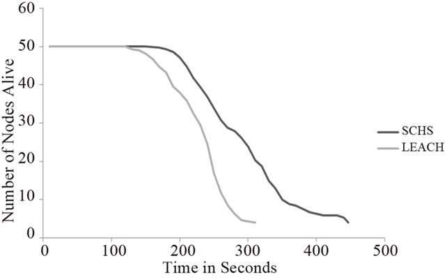
5.3.2. Node Death Rate
Figures 7(a)-(c) show the node death rate for SCHS and LEACH for the three topologies: 50 × 50 m2 with 50 nodes, 100 × 100 m2 with 100 nodes and 150 × 150 m2 with 200 nodes.
It can be seen from Figures 7(a)-(c) that node death rate of SCHS is lower than LEACH in all the three cases. As we have find from the Figures 6(a)-(c) that nodes are consuming less energy in case of SCHS, thereby resulting in lower death rate.
5.3.3. Network Lifetime
Figures 8(a)-(c) shows the comparative analysis of three parameters of network lifetime which are as follows: First Node Death, 50% Node Death and Network Lifetime (All Nodes Death).
From Figure 8(a) it can be seen that the time of first node death for SCHS is significantly higher than LEACH. As there is very few long distance intra-cluster communications resulting in less consumption of energy by the nodes. Figures 8(b), (c) shows that there is increase in network lifetime for SCHS in all three topologies. So SCHS performs significantly better than LEACH and prolong the network lifetime.

Figure 5. Effect of value of d on node death rate for 100 × 100 m2 with 100 nodes network.

Table 3. Number of nodes in Border area and Inner area for different value of d.
 (a)
(a)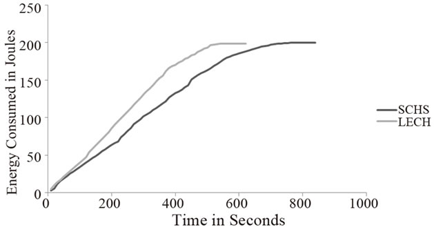 (b)
(b) (c)
(c)
Figure 6. (a) Energy consumption rate for 50 × 50 m2 with 50 nodes; (b) Energy consumption rate for 100 × 100 m2 with 100 nodes; (c) Energy consumption rate for 150 × 150 m2 with 200 nodes.
 (a)
(a) (b)
(b) (c)
(c)
Figure 7. (a) Node death rate for 50 × 50 m2 with 50 nodes; (b) Node death rate for 100 × 100 m2 with 100 nodes; (c) Node death rate for 150 × 150 m2 with 200 nodes.
 (a)
(a) (b)
(b) (c)
(c)
Figure 8. (a) First node death for three topologies; (b) 50% node death for three topologies; (c) Network lifetime for three topologies.
5.3.4. Data units received at Base Station
Figure 9 shows comparison of data units received at base station for LEACH and SCHS for all three topologies.
As analyzed from above figures that SCHS have better network lifetime, low energy consumption rate and low node death rate as LEACH that means SCHS have more network time to sense and send data to base station, it is also shown by Figure 9 that SCHS have more data units received at base station as compared to LEACH. So overall SCHS performs better than LEACH in terms of energy consumption rate, node death rate, network lifetime and data units received at base station.

Figure 9. Data units received at base station.
5.4. Simulation Summary
The SCHS approach outperforms the LEACH in prolonging the network lifetime with respect to three lifetime parameter which are first node death, 50% node death and all node death. The energy consumption rate and node death rate is low in case of SCHS because the nodes are conserving energy by having low intra-cluster communication distance. Because in case of SCHS network is performing for a longer time period, hence nodes have more time to sense the environment and for sending data to base station. So data units received at base station has been significantly improved in SCHS. SCHS does not require any global information because nodes are performing locally in distributed manner. SCHS can be implemented with any existing distributed clustering approach.
Wireless sensor networks are application specific networks and as mentioned have large application area. Proposed scheme, SCHS, works significantly for continuous data gathering application. In proposed scheme, border area nodes functions more time than inner area nodes, hence scheme is best applicable for critical surveillance monitoring applications.
6. Conclusions
Clustering algorithms are energy efficient approaches for wireless sensor networks as the algorithms reduces the communication distances and exploits data redundancy by data aggregation. Cluster head selection is an important issue for energy efficiency of clustering schemes. In this paper, a simple and easy to implement scheme for cluster head selection, SCHS, is introduced. The scheme can be implemented with any existing distributed clustering algorithm. SCHS partition the network into two parts: border area and inner area. Cluster head selection is restricted to nodes of inner area nodes. SCHS reduces the intra-cluster communication distance.
Simulation analysis shows that SCHS extended the lifetime of network as node death rate and energy consumption rate of nodes is low for SCHS as compared to LEACH. Also more data units are received at the base station in SCHS as compared to LEACH.
REFERENCES
- N. A. Pantazis and D. D. Vergados, “A Survey on Power Control Issues in Wireless Sensor Networks,” IEEE Communication Surveys, Vol. 9, No. 4, 2007, pp. 86-107. doi:10.1109/COMST.2007.4444752
- A. Arora, P. Dutta, S. Bapat, V. Kulathumani, H. Zhang, V. Naik, V. Mittal, H. Cao, M. Demirbas, M. Gouda, Y. Choi, T. Herman, S. Kulkarni, U. Arumugam, M. Nesterenko, A. Vora, and M. Miyashita, “A Line in the Sand: A Wireless Sensor Network for Target Detection, Classification, and Tracking,” Computer Network, Vol. 46, No. 5, 2004, pp. 605-634. doi:10.1016/j.comnet.2004.06.007
- H. Karl and A. Willig, “Protocols and Architectures for Wireless Sensor Networks,” John Wiley & Sons, Hoboken, 2007.
- A. Mainwaring, D. Culler, J. Polastre, R. Szewczyk and J. Anderson, “Wireless Sensor Networks for Habitat Monitoring,” Proceedings of the 1st ACM International Workshop on Wireless Sensor Networks and Applications, New York, 28 September 2002, pp. 88-97.
- A. Flammini, P. Ferrari, D. Marioli, E. Sisinni and A. Taroni, “Wired and Wireless Sensor Networks for Industrial Applications,” Journal of Microelectron, Vol. 40, No. 9, 2009, pp. 1322-1336. doi:10.1016/j.mejo.2008.08.012
- A. Milenkovi´c, C. Otto and E. Jovanov, “Wireless Sensor Networks for Personal Health Monitoring: Issues and an Implementation,” Computer Communication, Vol. 29, No. 13-14, 2006, pp. 2521-2533. doi:10.1016/j.comcom.2006.02.011
- I. F. Akyildiz, W. Su, Y. Sankarasubramaniam and E. Cayirci, “Wireless Sensor Networks: A Survey,” Computer Networks, Vol. 38, No. 4, 2002, pp. 393-422. doi:10.1016/S1389-1286(01)00302-4
- A. A. Abbasi and M. Younis, “A Survey on Clustering Algorithms for Wireless Sensor Networks,” Computer Communication, Vol. 30, No. 14-15, 2007, pp. 2826-2841. doi:10.1016/j.comcom.2007.05.024
- D. Wei and H. Chan, “Clustering Ad Hoc Networks: Schemes and Classifications,” Proceedings of the 3rd Annual IEEE Communications Society on Sensor and Ad Hoc Communications and Networks, Reston, 28 September 2006, pp. 920-926. doi:10.1109/SAHCN.2006.288583
- W. R. Heinzelman, A. Chandrakasan and H. Balakrishnan, “Energy-Efficient Communication Protocol for Wireless Microsensor Networks,” Proceedings of the 33rd Hawaii International Conference on System Sciences, Washington DC, 4-7 January 2000, pp. 1-10. doi:10.1109/HICSS.2000.926982
- C.-J. Jiang, W.-R. Shi, M. Xiang and X.-L. Tang, “Energy-Balanced Unequal Clustering Protocol for Wireless Sensor Networks,” Journal of China Universities of Posts and Telecommunications, Vol. 17, No. 4, 2010, pp. 94-99.
- F. Bajaber and I. Awan, “Adaptive Decentralized Reclustering Protocol for Wireless Sensor Networks,” Journal of Computer System Science, Vol. 77, No. 2, 2011, pp. 282-292. doi:10.1016/j.jcss.2010.01.007
- Q. Li, Q. X. Zhu and M. W. Wang, “Design of a Distributed Energy Efficient Clustering Algorithm for Heterogeneous Wireless Sensor Networks,” Computer Communications, Vol. 29, No. 12, 2006, pp. 2230-2237. doi:10.1016/j.comcom.2006.02.017
- D. Kumar, T. C. Aseri and R. B. Patel, “EEHC: Energy Efficient Heterogeneous Clustered Scheme for Wireless Sensor Networks,” Computer Communications, Vol. 32, No. 4, 2009, pp. 662-667. doi:10.1016/j.comcom.2008.11.025
- K. Fall and K. Vardhan, “The Network Simulator NS-2”. http:// www.isi.edu/nsnam/ns/
- D. C. Chinh, R. Kumar and S. K. Panda, “Optimal Data Aggregation Tree in Wireless Sensor Networks Based on Intelligent Water Drops Algorithm,” IET Wireless Sensor System, Vol. 2, No. 3, 2012, pp. 282-292. doi:10.1049/iet-wss.2011.0146
- M. Liu, J. Cao, G. Chen and X. Wang, “An EnergyAware Routing Protocol in Wireless Sensor Networks,” Sensors, Vol. 9, No. 1, 2009, pp. 445-462. doi:10.3390/s90100445