iBusiness
Vol.2 No.2(2010), Article ID:1952,7 pages DOI:10.4236/ib.2010.22014
Inventories and Mixed Duopoly with State-Owned and Labor-Managed Firms
![]()
Institute for Basic Economic Science, Osaka, Japan.
Email: ohnishi@e.people.or.jp
Received February 25th, 2010; revised April 2nd, 2010; accepted May 8th, 2010.
Keywords: Inventory investment, State-owned firm, Labor-managed firm
ABSTRACT
This paper considers a two-period mixed market model in which a state-owned firm and a labor-managed firm are allowed to hold inventories as a strategic device. The paper then shows that the equilibrium in the second period occurs at the Stackelberg point where the state-owned firm is the leader.
1. Introduction
The analysis of mixed market models that incorporate state-owned public firms has been performed by many researchers, such as [1-16].1 However, these studies consider mixed market models in which state-owned firms compete with profit-maximizing capitalist firms, and do not include labor-managed firms.
Mixed market models that incorporate labor-managed firms have also been studied by many researchers, such as [22-34].2 However, these studies consider mixed market models in which labor-managed firms compete against profit-maximizing capitalist firms, and do not include state-owned firms.
Some studies examine mixed market models with state-owned and labor-managed firms. For example, Delbono and Rossini [40] explore the creation of 1) a duopoly formed by a labor-managed firm and a state-owned firm in a Cournot-Nash setting, and 2) a horizontal merger between the same agents. In addition, Ohnishi [41] investigates the behaviors of a state-owned firm and a labormanaged firm in a two-stage mixed market model with capacity investment as a strategic instrument. There are few studies that examine mixed market models with state-owned and labor-managed firms.
Therefore, we consider a two-period mixed market model in which a state-owned firm and a labor-managed firm can hold inventories as a strategic device.3 In the first period, each firm simultaneously and independently chooses how much it sells in the current market and the level of inventory it holds for the second-period market. We analyze the equilibrium of the mixed duopoly model, and show that the equilibrium in the second period occurs at the Stackelberg point where the state-owned firm is the leader.
The remainder of this paper is organized as follows. In Section 2, we describe the model. Section 3 gives supplementary explanations of the model. Section 4 analyzes the equilibrium of the model. Section 5 concludes the paper. All proofs are given in the appendix.
2. The Model
Let us consider a mixed market with one state-owned welfare-maximizing firm (firm 1) and one labor-managed profit-per-worker-maximizing firm (firm 2), producing perfectly substitutable goods. There is no possibility of entry or exit. In the remainder of this paper, subscripts 1 and 2 refer to firms 1 and 2, respectively, and superscripts 1 and 2 refer to periods 1 and 2, respectively. In addition, when  and
and  are used to refer to firms in an expression, they should be understood to refer to 1 and 2 with
 . The price of each period is determined by
 , where
  is the aggregate sales of each period. We assume that
  and
and . The game runs as follows. In the first period, each firm simultaneously and independently chooses its first-period production
  and its first-period sales
 . Firm
 ’s inventory
  becomes
 . At the end of the first period, firm
  knows
knows  and
and . In the second period, each firm simultaneously and independently chooses its second-period production
 . At the end of the second period, each firm sells
  and holds no inventory. For notational simplicity, we consider the game without discounting.
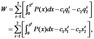
Since , social welfare is
 (1)
(1)
where  denotes firm
 ’s constant marginal cost. The demand and cost conditions that firms face remain unchanged over time. We assume that firm 1 is less efficient than firm 2, i.e.
 .4 We define
 (2)
(2)
Furthermore, since , firm 2’s profit per worker is
 (3)
(3)
where  is firm 2’s fixed cost, and
 ![]() is the amount of labor in firm 2. We assume that
is the amount of labor in firm 2. We assume that ![]() is the function of
is the function of  with
with  and
and . This assumption means that the marginal quantity of labor used is increasing. We define
 (4)
(4)
We analyze the subgame perfect Nash equilibrium of the mixed market model.
3. Supplementary Explanation
In this section, we give supplementary explanations of the model described in the previous section. First, we derive firm 1’s reaction functions from (2). In the first period, since there is no inventory available, firm 1’s reaction function is defined by
 (5)
(5)
In the second period, firm 1’s reaction function without inventory is defined by
 (6)
(6)
and thus its best response is shown as follows:
 (7)
(7)
Firm 1 maximizes social welfare with respect to , given
 . When the inventory is zero, the first-order condition for firm 1 is
 (8)
(8)
Furthermore, we have
 (9)
(9)
In the first period, the slope of the reaction function of firm 1 is –1. In the second period, the slope of the best response of firm 1 is –1 for , and it is zero for
 . This means that firm 1 treats
  as strategic substitutes.5
Second, we derive firm 2’s reaction functions from (4). In the first period, since there is no inventory available, firm 2’s reaction function is defined by
 (10)
(10)
In the second period, firm 2’s reaction function without inventory is defined by
 (11)
(11)
and thus its best response is shown as follows:
 (12)
(12)
Firm 2 maximizes its profit per worker with respect to , given
 . The equilibrium must satisfy the following conditions: When the inventory is zero, the first-order condition for firm 2 is
 (13)
(13)
and the second-order condition is
 (14)
(14)
Furthermore, we have
 (15)
(15)
Since ,
,  , so that
 is positive; that is,
  is upward sloping. This means that firm 2 treats
  as strategic complements.
Third, we consider Stackelberg games. If firm 1 is the Stackelberg leader, then firm 1 selects , and firm 2 selects
  after observing
 . Firm 1 maximizes
  with respect to
 . On the other hand, if firm 2 is the Stackelberg leader, then firm 2 selects
 , and firm 1 selects
  after observing
 . Firm 2 maximizes
  with respect to
 . We present the following lemma:
Lemma 1. Each firm’s Stakelberg leader sales exceed its Cournot sales without inventory.
Lemma 1 means that each firm prefers sales higher than its Cournot sales without inventory.
4. Equilibrium
In this section, we analyze the equilibrium outcomes of the mixed market model. The equilibrium in the first period is stated by the following proposition:
Proposition 1. In the first-period of the mixed market model, the equilibrium coincides with the Cournot Nash solution without inventory .
.
The intuition behind Proposition 1 is as follows. There is no inventory available in the first period, and further  does not affect
  and
and . Since
  and
and  decrease by deviating from the Cournot Nash solution, each firm has no incentive to do so, and therefore the equilibrium is at
 .
.
We now consider the equilibrium of the second period. It is thought that the equilibrium of the second period is decided by the level of . We discuss the following three cases:
1) The case in which only firm 1 can hold inventory 2) The case in which only firm 2 can hold inventory 3) The case in which each firm can hold inventory We discuss these cases in order.
1) The case in which only firm 1 can hold inventory First, consider Figure 1, where  denotes firm
 ’s second-period reaction curve without inventory.
  is downward sloping, whereas
  is upward sloping. Suppose that firm 1 holds
  in the second period. By holding inventory, firm 1’s best response becomes (7). Firm 1’s inventory investment thus creates a kink in its reaction curve at the level of
 . That is, firm 1’s reaction curve becomes the kinked bold lines as drawn in the figure. The equilibrium is decided in a Cournot fashion, i.e., the intersection of firm 1’s and firm 2’s reaction curves gives us the equilibrium of the game. Figure 1 shows that the intersection of new reaction curves is not affected by the kink. Hence, the equilibrium occurs at
 .
.
Next, consider Figure 2. Suppose that firm 1 holds . From (7), firm 1’s reaction curve becomes the kinked bold lines. The intersection of firm 1’s and firm 2’s reaction curves gives us the equilibrium of the game.

Figure 1. The equilibrium occurs at N

Figure 2. The equilibrium occurs at B
From Figure 2, we see that the inventory level of  changes the equilibrium of the game. The intersection of the new reaction curves is the equilibrium sales in the second period. That is, if firm 1 holds
 , then the equilibrium occurs at
 .
.
We can now state the following proposition:
Proposition 2. Suppose that only firm 1 can hold inventory. Then the equilibrium coincides with the Stackelberg solution where firm 1 is the leader.
2) The case in which only firm 2 can hold inventory First, consider Figure 3. Suppose that firm 2 holds . From (12), firm 2’s reaction curve becomes the kinked bold broken lines. In this figure, the reaction curves of both firms do not cross each other. That is, if firm 2 maintains the inventory level of
 , then there is no solution.
Next, consider Figure 4. Suppose that firm 2 holds . From (12), firm 2’s reaction curve becomes the kinked bold broken lines. The reaction curves of both firms cross twice as in Figure 4. We can see easily that
  and
and  are stable solutions. That is, there are two stable solutions. However, we see that firm 2’s profit per worker is higher at
  than at
 .
.
We can now state the following proposition:
Proposition 3. Suppose that only firm 2 can hold inventory. Then the equilibrium coincides with the Cournot Nash solution without inventory .
.
3) The case in which each firm can hold inventory First, consider Figure 5. Suppose that firms 1 and 2 hold  and
and , respectively. In this figure, the reaction curves of both firms do not cross each other. That is, if firms 1 and 2 maintain the inventory levels of
  and
and , respectively, then there is no solution.

Figure 3. The reaction curves do not cross each other
Next, consider Figure 6. Suppose that each firm holds . Firm 1’s reaction curve becomes the kinked bold

Figure 4. The reaction curves cross twice

Figure 5. The new reaction curves do not cross each other

Figure 6. The new reaction curves cross twice
lines, and firm 2’s reaction curve becomes the kinked bold broken lines. The new reaction curves of both firms cross twice. We see easily that  and
and ![]() are stable solutions. That is, there are two stable solutions. However, we see that firm 2’s profit per worker is higher at
are stable solutions. That is, there are two stable solutions. However, we see that firm 2’s profit per worker is higher at  than at these points.
The main result of this study is described by the following proposition:
Proposition 4. In the second period of the mixed market model, the equilibrium coincides with the Stackelberg solution where firm 1 is the leader. At equilibrium, firm 2’s profit per worker is lower than in the Cournot mixed duopoly game without inventory.
5. Conclusions
We have considered a two-period mixed market model in which a state-owned firm and a labor-managed firm are allowed to hold inventories as a strategic device. We have then shown that the equilibrium in the second period occurs at the Stackelberg point where the stateowned firm is the leader and at equilibrium the labormanaged firm’s profit per worker is lower than in the Cournot mixed duopoly game without inventory. As a result, we see that the introduction of inventory investment into the analysis of mixed market competition with state-owned and labor-managed firms is profitable for the state-owned firm while it is not profitable for the labor-managed firm.
REFERENCES
- F. Delbono and V. Denicolò, “Regulating Innovative Activity: The Role of Public Firm,” International Journal of Industrial Organization, vol. 11, no. 1, March 1993, pp. 35-48.
- L. Nett, “Why Private Firms are more Innovative than Public Firms,” European Journal of Political Economy, vol. 10, no. 4, December 1994, pp. 639-653.
- J. Willner, “Welfare Maximization with Endogenous Average Costs,” International Journal of Industrial Organization, vol. 12, no. 3, September 1994, pp. 373-386.
- K. Fjell and D. Pal, “A Mixed Oligopoly in the Presence of Foreign Private Firms,” Canadian Journal of Economics, vol. 29, no. 3, August 1996, pp. 737-743.
- K. George and M. La Manna, “Mixed Duopoly, Inefficiency, and Public Ownership,” Review of Industrial Organization, vol. 11, no. 6, December 1996, pp. 853-860.
- M. D. White, “Mixed Oligopoly, Privatization and Subsidization,” Economics Letters, vol. 53, no. 2, November 1996, pp. 189-195.
- S. Mujumdar and D. Pal, “Effects of Indirect Taxation in a Mixed Oligopoly,” Economics Letters, vol. 58, no. 2, February 1998, pp. 199-204.
- D. Pal, “Endogenous Timing in a Mixed Oligopoly,” Economics Letters, vol. 61, no. 2, November 1998, pp. 181-185.
- D. Pal and M. D. White, “Mixed Oligopoly, Privatization, and Strategic Trade Policy,” Southern Economic Journal, vol. 65, no. 2, April 1998, pp. 264-281.
- J. Poyago-Theotoky, “R & D Competition in a Mixed Duopoly under Uncertainty and Easy Imitation,” Journal of Comparative Economics, vol. 26, no. 3, September 1998, pp. 415-428.
- A. Nishimori and H. Ogawa, “Public Monopoly, Mixed Oligopoly and Productive Efficiency,” Australian Economic Papers, vol. 41, no. 2, June 2002, pp. 185-190.
- J. C. Bárcena-Ruiz and M. B. Garzón, “Mixed Duopoly, Merger and Multiproduct Firms,” Journal of Economics, vol. 80, no. 1, August 2003, pp. 27-42.
- T. Matsumura, “Stackelberg Mixed Duopoly with a Foreign Competitor,” Bulletin of Economic Research, vol. 55, no. 3, July 2003, pp. 275-287.
- K. Ohnishi, “A Mixed Duopoly with a Lifetime Employment Contract as a Strategic Commitment,” FinanzArchiv, vol. 62, no. 1, March 2006, pp. 108-123.
- J. C. Bárcena-Ruiz, “Endogenous Timing in a Mixed Duopoly: Price Competition,” Journal of Economics, vol. 91, no. 3, July 2007, pp. 263-272.
- J. Fernández-Ruiz, “Managerial Delegation in a Mixed Duopoly with a Foreign Competitor,” Economics Bulletin, vol. 29, no. 1, February 2009, pp. 90-99.
- D. Bös, “Public Enterprise Economics,” Dieter Bos, North-Holland, 1986.
- D. Bös, “Privatization: A Theoretical Treatment,” Clarendon Press, Oxford, 2001.
- J. Vickers and G. Yarrow, “Privatization: An Economic analysis,” MIT Press, Cambridge, 1988.
- H. Cremer, M. Marchand and J.-F. Thisse, “The Public firm as an Instrument for Regulating an Oligopolistic Market,” Oxford Economic Papers, vol. 41, no. 1, January 1989, pp. 283-301.
- L. Nett, “Mixed Oligopoly with Homogeneous Goods,” Annals of Public and Cooperative Economics, vol. 64, no. 3, July 1993, pp. 367-393.
- C. Mai and H. Hwang, “Export Subsidies and Oligopolistic Rivalry between Labor-Managed and Capitalist Economies,” Journal of Comparative Economics, vol. 13, no. 3, September 1989, pp. 473-480.
- I. Horowitz, “On the Effects of Cournot Rivalry between Entrepreneurial and Cooperative Firms,” Journal of Comparative Economics, vol. 15, no. 1, March 1991, pp. 115-121.
- K. Okuguchi, “Labor-Managed and Capitalistic Firms in International Duopoly: The Effects of Export Subsidy,” Journal of Comparative Economics, vol. 15, no. 3, September 1991, pp. 476-484.
- H. Cremer and J. Crémer, “Duopoly with Employee-Controlled and Profit-Maximizing Firms: Bertrand vs. Cournot Competition,” Journal of Comparative Economics, vol. 16, no. 2, June 1992, pp. 241-258.
- G. Stewart, “Management Objectives and Strategic Interactions among Capitalist and Labour-Managed Firms,” Journal of Economic Behavior and Organization, vol. 17, no. 3, May 1992, pp. 423-431.
- E. Askildsen and N. J. Ireland, “Human Capital, Property right, and Labour Managed Firms,” Oxford Economic Papers, vol. 45, no. 2, April 1993, pp. 229-242.
- N. J. Ireland and G. Stewart, “On the Sale of Production Rights and Firm Organization,” Journal of Comparative Economics, vol. 21, no. 3, December 1995, pp. 289-307.
- K. Futagami and M. Okamura, “Strategic Investment: The Labor-Managed Firm and the Profit-Maximizing Firm,” Journal of Comparative Economics, vo. 23, no. 1, August 1996, pp. 73-91.
- H. M. Neary and D. Ulph, “Strategic Investment and the Co-Existence of Labour-Managed and Profit-Maximising Firms,” Canadian Journal of Economics, vol. 30, no. 2, May 1997, pp. 308-328.
- L. Lambertini and G. Rossini, “Capital Commitment and Cournot Competition with Labour-Managed and ProfitMax-Imising Firms,” Australian Economic Papers, vol. 37, no. 1, March 1998, pp. 14-21.
- L. Lambertini, “Spatial Competition with Profit-Maximising and Labour-Managed Firms,” Papers in Regional Science, vol. 80, no. 4, October 2001, pp. 499-507.
- K. Ohnishi, “Strategic Investment in a New Mixed Market with Labor-Managed and Profit-Maximizing Firms,” Meto-economica, vol. 59, no. 4, November 2008, pp. 594-607.
- T. Cuccia and R. Cellini, “Workers’ Enterprises and the Taste for Production: The Arts, Sport and Other Cases,” Scottish Journal of Political Economy, vol. 56, no. 1, February 2009, pp. 123-137.
- B. Ward, “The Firm in Illyria: Market Syndicalism,” American Economic Review, vol. 48, no. 4, 1958, pp. 566-589.
- J. Ireland and P. J. Law, “The Economics of Labor-Managed Enterprises,” St. Martin’s Press, Macmillan, 1982.
- F. H. Stephan, Ed., “The Performance of Labour-Managed Firms,” Macmillan Press, Macmillan, 1982.
- J. P. Bonin and L. Putterman, “Economics of Cooperation and the Labor-Managed Economy,” Harwood Academic Publishers, Graubünden, 1987.
- L. Putterman, “Labour-Managed Firms,” In: S. N. Durlauf and L. E. Blume, Eds., The New Palgrave Dictionary of Economics, Palgrave Macmillan, Vol. 4, No. 1, 2008, pp. 791-795.
- F. Delbono and G. Rossini, “Competition Policy vs. Horizontal Merger with Public, Entrepreneurial, and LaborManaged Firms,” Journal of Comparative Economics, vol. 16, no. 2, June 1992, pp. 226-240.
- K. Ohnishi, “Capacity Investment and Mixed Duopoly with State-Owned and Labor-Managed Firms,” Annals of Economics and Finance, vol. 10, no. 1, May 2009, pp. 49-64.
- J. J. Rotemberg and G. Saloner, “The Cyclical Behavior of Strategic Inventories,” Quarterly Journal of Economics, vol. 104, no. 1, February 1989, pp. 73-97.
- T. Matsumura, “Cournot Duopoly with Multi-Period Competition: Inventory as a Coordination Device,” Australian Economic Papers, vol. 38, no. 3, September 1999, pp. 189-202.
- M. Gunderson, “Earnings Differentials between the Public and Private Sectors,” Canadian Journal of Economics, vol. 12, no. 2, May 1979, pp. 228-242.
- J. I. Bulow, J. D. Geanakoplos and P. D. Klemperer, “Multimarket Oligopoly: Strategic Substitutes and Complements,” Journal of Political Economy, vol. 93, no. 3, June 1985, pp. 488-511.
Appendix
Proof of Lemma 1
First, we prove that firm 1’s Stakelberg leader sales are higher than its Cournot sales without inventory. Firm 1 maximizes  with respect to
 . Therefore, firm 1’s Stackelberg leader sales satisfy the firstorder condition:
 , (16)
where  is positive from (8) and
 , and
, and  is also positive from (10), (11) and (15). To satisfy (16),
  must be negative.
Second, we prove that firm 2’s Stakelberg leader sales are higher than its Cournot sales without inventory. Firm 2 maximizes  with respect to
 . Therefore, firm 2’s Stackelberg leader sales satisfy the first-order condition:
 , (17)
where  is negative from
 , and
, and  is also negative from (5), (6) and (9). To satisfy (17),
  must be negative. Thus, the lemma follows. Q. E. D.
Proof of Proposition 1
Since  does not affect
  and
and ,
,  has no strategic value. Thus, the result follows easily from (5) and (10). Q. E. D.
Proof of Proposition 2
The equilibrium is decided in a Cournot fashion, i.e., the intersection of firm 1’s and firm 2’s reaction functions gives us the equilibrium of the game. In , social welfare is the highest at firm 1’s Stakelberg leader point. Lemma 1 states that firm 1’s Stakelberg leader sales exceed its Cournot sales without inventory.
  is downward sloping, whereas
  is upward sloping. From (7), we see that the equilibrium in the second period is decided by the value of
 .
.  can take values of zero and above. Our equilibrium concept is the subgame perfect equilibrium and all information in the model is common knowledge. In the first period, firm 1 chooses
 associated with its second-period Stackelberg leader solution. Thus, Proposition 2 follows. Q. E. D.
Proof of Proposition 3
Lemma 1 states that firm 2’s Stakelberg leader sales exceed its Cournot sales without inventory.  is downward sloping, whereas
  is upward sloping. From (12), if
 , then it is impossible for firm 2 to change
  in equilibrium. That is, if
 , then inventory does not function as a strategic device. Let
  be assumed to be continuous and concave in
 . The further a point on
  gets from firm 2’s Stackelberg leader point, the more firm 2’s profit per worker decreases. Thus, Proposition 3 follows Q. E. D.
Proof of Proposition 4
First, consider the possibility that firm 2 holds inventory as a strategic device. Lemma 1 states that firm 2’s Stakelberg leader sales exceed its Cournot sales without inventory.  is downward sloping, whereas
  is upward sloping. From (12), firm 2 cannot choose its Stackelberg leader point. Let
  be assumed to be continuous and concave in
 . The further a point on
  gets from firm 2’s Stackelberg leader point, the more firm 2’s profit per worker decreases. Hence, firm 2 does not choose
 . If
. If  and
and , then there is no solution. If
  and
and , then the solution becomes
 . However, at solution, firm 2’s profit per worker is lower than in the Cournot mixed duopoly game without inventory. Hence, firm 2 does not hold inventory as a strategic device whether firm 1 holds inventory or not.
Next, consider the possibility that firm 1 holds inventory as a strategic device. Our equilibrium concept is the subgame perfect equilibrium and all information in the model is common knowledge. Hence, firm 1 knows that firm 2 does not hold inventory as a strategic device whether firm 1 holds inventory or not. Lemma 1 states that firm 1’s Stakelberg leader sales exceed its Cournot sales without inventory. From (7), we see that the equilibrium in the second period is decided by the value of .
.  can take values of zero and above. In the first period, firm 1 chooses
  associated with its second-period Stackelberg leader solution. Thus, the equilibrium coincides with the Stackelberg solution where firm 1 is the leader.
NOTES
1See [17-21] for excellent surveys.
2The pioneering work on a theoretical model of a labor-managed firm is conducted by Ward [35]. See also [36-39] for excellent surveys.
3For private market models with inventories as a strategic device, see Rotemberg and Saloner [42] and Matsumura [43].
4This assumption is justified in Nett [2,21] and Gunderson [44], and is often used in literature studying mixed markets. See, for instance, George and La Manna [5], Mujumdar and Pal [7], Pal [8], Nishimori and Ogawa [11], Matsumura [13], Ohnishi [14], and Fernández-Ruiz [16]. If firm 1 is equally or more efficient than firm 2, then firm 1 chooses ![]() and
and  such that price equals marginal cost. Therefore, firm 2 has no incentive to operate in the market, and firm 1 supplies the entire market, resulting in a social-welfare-maximizing public monopoly. This assumption is made to eliminate such a trivial solution.
5The concepts of strategic substitutes and complements are due to Bulow, Geanakoplos, and Klemperer [45].