Engineering
Vol. 3 No. 11 (2011) , Article ID: 8658 , 8 pages DOI:10.4236/eng.2011.311134
Performance of a New Method of Multicomponent Images Segmentation in the Presence of Noise
1Laboratoire d’Instrumentation, d’Image et de Spectroscopie (L2IS), Institut National Polytechnique Félix Houphouët-Boigny (INPHB), Yamoussoukro, Côte d’Ivoire
2Laboratoire d’Ingénierie des Systèmes Automatisés (LISA), Institut Universitaire de Technologie d’Angers, Angers, France
E-mail: sie_ouat@yahoo.fr
Received August 23, 2011; revised October 11, 2011; accepted October 24, 2011
Keywords: multicomponent images, segmentation, n-D compact histogram, additional noise, Gaussian noise, Uniform noise, Correlated noise
ABSTRACT
Any undesirable signal limiting to a degree or another the integrity and the intelligibility of a useful signal can be considered as noise. In the general rule, the good performance of a system is assured only if the level of power of the useful signal exceeds by several orders of magnitude that of the noise (signal to noise of a several tens of decibels). However certain elaborate methods of treatment allow working with very low signal to noise ratio in an optimal way any a priori knowledge available on the signal useful to interpret. In this work, we evaluate the robustness of the noise on a new method of multicomponent image segmentation developed recently. Two types of additional noises are considered, which are the Gaussian noise and the uniform noise, with varying correlation between the different components (or planes) of the image. Quantitative results show the influence of the noise level on the segmentation method.
1. Introduction
Multicomponent images are composed of several plans of images. We can classify them into three main categories [1]: 1) The images of homogeneous components are those consisted of series of images of the same nature, and representing the same scene. The nature of the third dimension depending on the application may be temporal or polarimetric. 2) The images with quasi-homogeneous components are images intrinsically vectorial. Each pixel is characterized by the vector “color” or multispectral. The components are expressed numerically with the same measuring unit, for example energies in different wavebands. The only rigorous approach to treat such images is the vectorial approach. This work interests particularly this category of images. 3) The images with heterogeneous or multiprotocol components are images whose components are not the same nature because the different components of the image are obtained by the use of sources of different nature.
In a multicomponent image, a pixel can be considered as a vector of attributes of n elements (tuple, where n is the number of components of the image) from which each value of the tuple is resulting from a component of the image. Segmenting the images according to their radiometric attributes can be achieved by analyzing multidimensional histogram [2,3]. However, to manipulate a nD histogram (n > = 3) is not easy task because it requires a large memory [4-6]. The difficulty can be overcome by using a compact multidimensional histogram [7-12]. We have recently proposed a segmentation method [3] based on the analysis of compact nD histogram. We report here how this algorithm proves to be robust to additional noise considered as a harmful corrupting signal with the extraction of the useful signal.
In this work, we first make a brief presentation of our segmentation algorithm, for more details refer to the article [3]. Then we present here the additive noises that are likely considered Gaussian, uniform and so correlated. Finally the robustness of the noise is evaluated on a multicomponent synthetic image whose properties are described.
2. Algorithm of Multicomponent Images Segmentation
The classification of “colours” is carried out in two steps [3]: the learning step and the decision step.
The learning step is a hierarchical decomposition of populations in the compact n-D histogram. For each level of population pn, peaks Pi are identified by the FCCL algorithm for a given value of α, which retains the connected components whose populations are greater than or equal to pn. Each peak is then iteratively decomposed into narrower peaks, beginning from population 0. A peak is labelled as significant if it represents a population greater than or equal to a threshold S (expressed in percent of the total population in the histogram). The procedure is illustrated in part (a) of Figure 2 (drawn in one dimension for clarity). We shall name kernels Ki the peaks corresponding to circled leaves in part (b) of Figure 1. In other words, kernels are significant peaks (part a of figure 1) without descendants in the hierarchical decomposition tree (part (b) of Figure 1) (e.g., Figure 1 shows five significant peaks Pi (i = 0 to 4) and three kernels Ki (i = 2, 3, 4)). The number of classes Nc is taken equal to the number of kernels (the class corresponding to kernel Ki is noted Ci). Therefore Nc depends on the threshold S, i.e. on the precision the image colors are analyzed with and the value of α the degree of similarity between the spels.
At the decision step, the mass center µ(Ki) of each kernel Ki is calculated in the feature multidimensional space. Let us denote by ß the color corresponding to the point of coordinates (g1, g2, ∙∙∙, gn) in the feature space. Two cases appear: if (g1, g2, ∙∙∙, gn) belongs to Ki, color ß is attributed to class Ci; if not, let us denote by Pk the peak which belong to (g1, g2, ∙∙∙, gn); color ß is attributed to class Ci corresponding to kernel Ki, son of Pk, knowing that d[µ(Ki), (g1, g2, ∙∙∙, gn)] is minimum, where d[y, z] is the Euclidean distance between y and z.
This method calls HierarchieFuzzy_nD.
Figure 2 shows an example of segmented image of the probe image, inspired by the image Savoise [2,14].
3. Synthetic Image and Additional Noise
There are many sources of noise to an image, for example in the case of a Gaussian random variable, or Gaussian noise can be added by the system to the ideal image. For digital images, the source is the precision of the CCD or CMOS highlighted by a high gain [13,14]. Two types of noise are considered in this work.
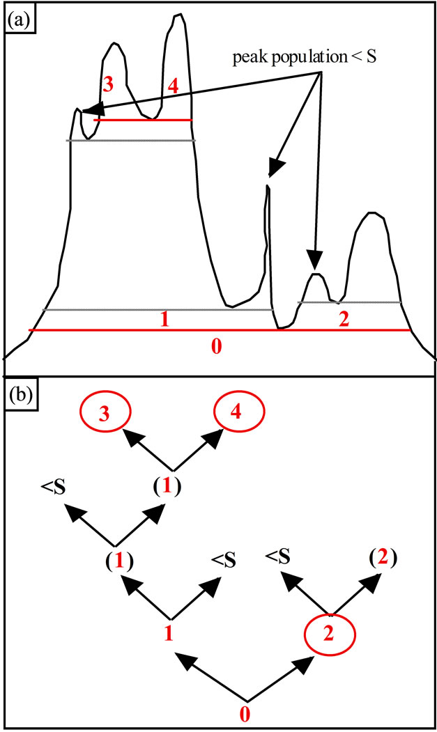
Figure 1. An example of hierarchical decomposition with α = 0.5. The circled leaves (part (b)) correspond to significant peaks as obtained at the end of the iterative decomposition (solid lines in part (a)), whereas leaves marked < S (part (b)) correspond to insignificant peaks (dotted lines in part (a)).
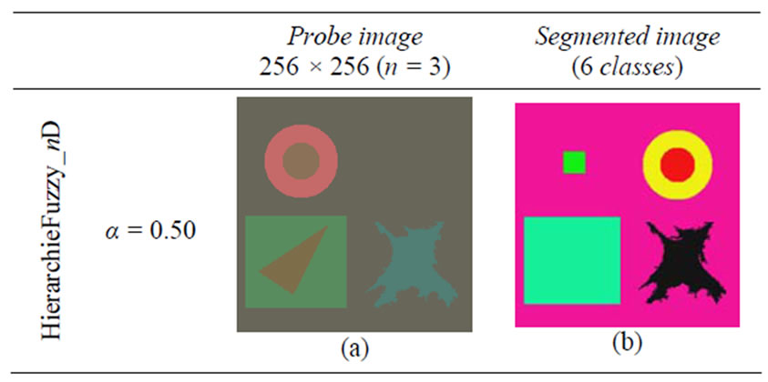
Figure 2. Example of segmented image by HierarchieFuzzy_ nD.
3.1. Synthetic Image
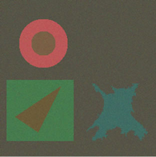
The probe image (Figure 2(a)) is a synthetic RGB color image coded on 24 bits, with a 256 × 256 resolution. It is inspired by the image Savoise [2,15]. This image (noiseless) is composed of six regions with different geometrical shapes and pure colors as indicated in table 1. The six classes are numbered as shown in Figure 3.
For segmenting the probe image (Figure 3) into 2 to 6 classes, the choice of the intervals of the threshold S is given by Table 2.
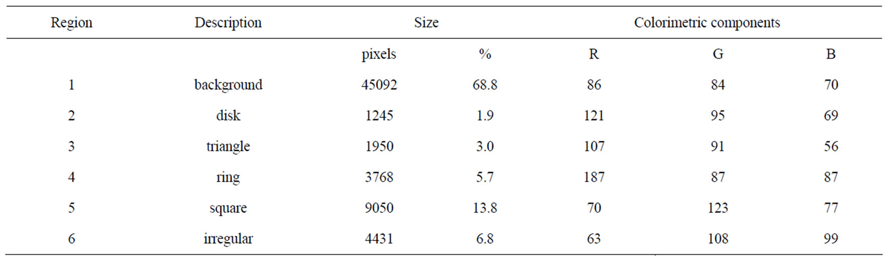
Table 1. Characteristics of the noiseless probe image.

Table 2. Intervals of threshold S for a class number desired.
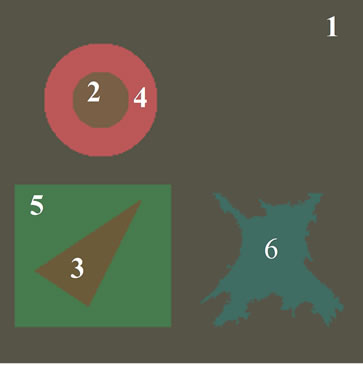
Figure 3. probe image with six numbered regions.
3.2. Additional Gaussian Noise
Also called Normal distribution, it occurs very frequently in statistics, advanced sciences like photonics, electronics, transmission, quantum mechanics and economics and can be used to approximate many distributions occurring in nature and in the manmade world. For example, the white noise in telecommunication due to the resistance, amplifier, transistor and diode. The theory of normal distribution also finds use in natural and social sciences.
In the images, the source is the precision of the sensor CCD or CMOS highlighted by a high gain [13,14]. The normal distribution can be characterized by the mean and standard deviation. The mean is generally represented by μ and the standard deviation by σ. For a perfect normal distribution, the mean, median and mode are all equal. The normal distribution function can be written in terms of the mean and standard deviation as follows:
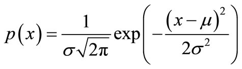 (1)
(1)
The simplest case of a normal distribution is known as the standard normal distribution (μ = 0 and σ = 1), described by the probability density p(x):
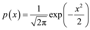 (2)
(2)
The normal distribution is usually denoted by  . Thus when a random variable Z is distributed normally with mean μ and variance σ2, we write Z ~
 .
.
We suppose that X follows the distribution  and we pose
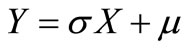 , then Y follows the distribution
 .
.
Our developments have been realized in the Matlab environment. The function (algorithm) for generating a 2D (or image) Gaussian noise with 256 × 256 resolution name Gnoise is given below. Figure 4 shows the probe image corrupted with an additional Gaussian noise and its segmentation by HierarchieFuzzy_nD.
function Gn = Gnoise(μ, σ)
% generating a Gaussian noise with for example
% 2D (or image) Gaussian noise Gn with standard deviation σ and mean μ
Gn = σ*randn(256,256) + μ ;
% End of the function
3.3. Additional Uniform Noise
In probability theory, discrete uniform law is a discrete probability law which can be characterized by saying that each value of a finite set of possible values is equally likely to occur (we speak of equal probability).
A random variable that can take n possible values K1, K2, ∙∙∙, Kn following a uniform distribution when the probability of any value Ki is defined by:
 (a)
(a)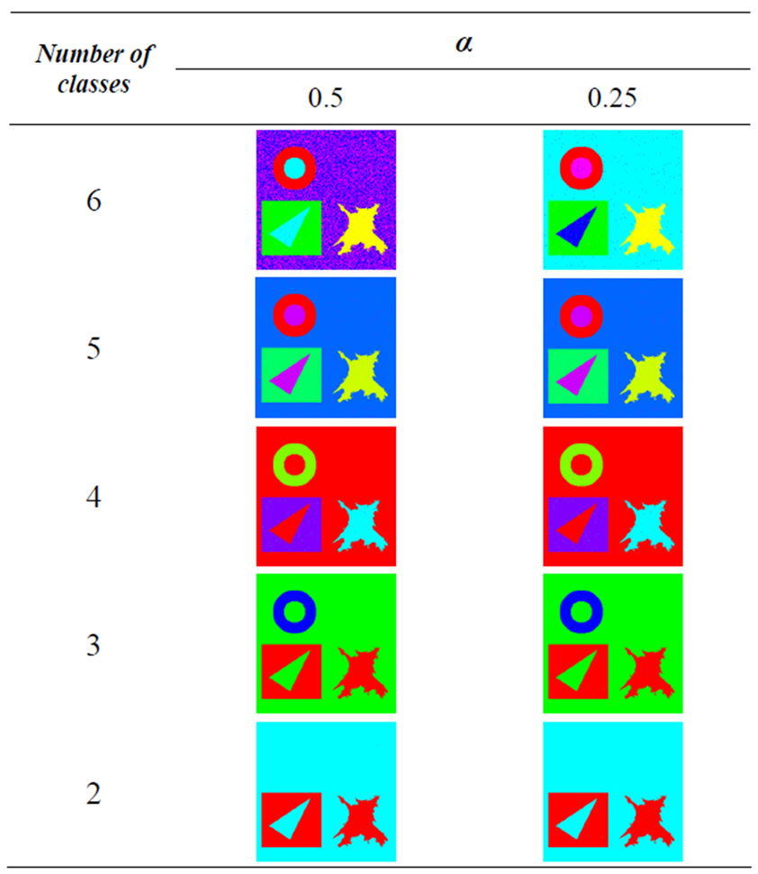 (b)
(b)
Figure 4. The probe image corrupted with a Gaussian noise of σ = 0.02 (a) and its segmentation for α = 0.5 and α = 0.25 by HierarchieFuzzy_nD (b).
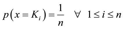 (3)
(3)
The function for generating a 2D (or image) Uniform noise with 256 × 256 resolution name Unoise is given below; Figure 4 shows the probe image corrupted with an additional Uniform noise.
function Un = Unoise(μ, σ)
% generating a Uniform noise
% 2D (or image) Uniform noise Un with standard deviation σ and mean μ
Un = σ*rand(256,256) + μ ;
% End of the function
3.4. Additional Correlated Noise
In order to evaluate the robustness of our segmentation method, the different components of the probe image have been corrupted by additional Gaussian or Uniform noises with more or less correlation. The noise generation has been realized by using Matlab language.
Being Nm1, Nm2, ∙∙∙, Nmn n (n >= 3) matrices of marginal center noise, and Nc a matrix of common centered noise, with the same standard deviation σ, the alteration of an image constituted of the n spectral components P1, P2, ∙∙∙, Pn is given by :
PiN = Pi + βNc + (1 − β)Nmi (i = 1, 2, ∙∙∙, n) (4)
where the noise correlation can be adjusted through β, from uncorrelated noise (β = 0) to totally correlated noise (β = 1). A partially correlated noise corresponds to β = 0.5.
An example of a corrupted image is given on Figure 4(a) or Figure 5. It is obtained from Figure 3 by adding uncorrelated Gaussian noise or Uniform noise with σ = 0.02.
When we apply to the noiseless probe image (Figure 3) the segmentation algorithm Hierarc-hieFuzzy_nD, it provides a class number which grows from 1 to 6 when the threshold S (Figure 1) which decreases from 100% to 0%. The classes so obtained will be taken as references of segmented images for calculating the segmentation errors induced by adding noise into the original probe image. The following figure (Figure 6) presents the probe image corrupted with a partially correlated Gaussian noise and its segmentation into six classes.
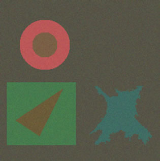
Figure 5. The probe image corrupted with an Uniform noise of σ = 0.02.
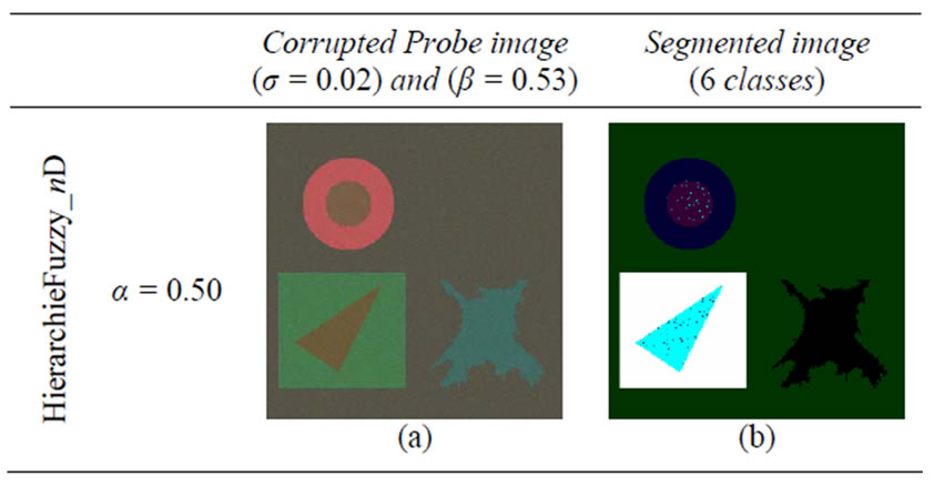
Figure 6. Corrupted probe image with a partially correlated Gaussian noise (σ = 0.02) and its segmentation.
4. Evaluation of Segmentation Errors Due to the Noise
The measure of Vinet [16-19] is a supervised criterion which corresponds to the correct segmentation or classification rate between segmentation result and reference segmentation. For synthetic image, the ground truth is available. This criterion is often used to compare a segmentation result  with a ground truth
  in the literature. We compute the following superposition table:
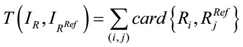 (5)
(5)
where 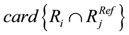 is the number of pixels resulting from the intersection of regions
  and
and  in the ground truth. The best match between
  and
and  is one that maximizes
 . Vinet’s measure gives a dissimilarity measure, it is computed as follows:
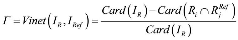 (6)
(6)
For a given number Nc of classes in noiseless image (2 ≤ Nc ≤ 6) , the classification will be considered as robust to noise if first Nc classes can be found in the corrupted image (for the two images the threshold S providing Nc classes will be eventually different). In our case, we associate the regions between  and
and  respectively to the classes
  and
and . In this case the regions are paired by minimizing accordance to the Equation (4) the quantity:
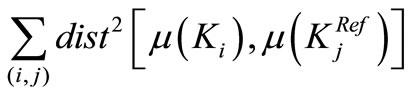 (7)
(7)
where dist represents the Euclidian distance. The minimization considers the kernels mass centers rather than the classes mass centers in order to make pairing independent of the classification decision step.
The measure г so calculated is more relevant to the segmentation by classification than the general measure of Vinet [16-19].
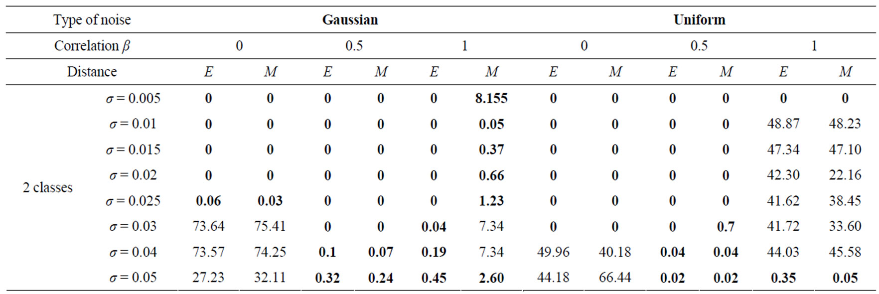
The classification error Г has been measured for the probe image of figure 3, altered with Gaussian or Uniform noise. The noise correlation between the R, G, B planes is realized using the parameter β. Three β values are considered: β = 0 (uncorrelated noise), β = 0.5 (partially correlated noise) and β = 1 (totally correlated noise). Eight values of noise standard deviation are applied (from σ = 0.005 to σ = 0.05). The distance used used for attributing pixels to different classes is either the Euclidian distance (E) or the Mahalanobis (M). The threshold S is adjusted so as to obtain 2, 3, 4, 5 or 6 classes. Sometimes, there are some cases where S adjustment does not allow obtaining the desired class number.
5. Results and Discussion
5.1. Robustness of Our Segmentation Method in the Presence of Noise and the Effect of Noise on the Class Number
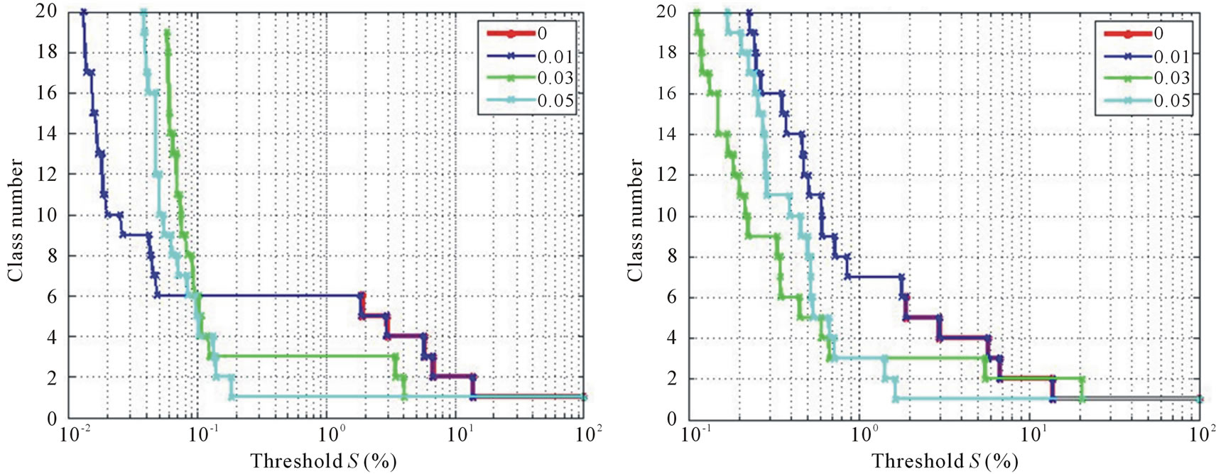
In a general way, to estimate the robustness of our segmentation at a number of classes varying from 2 to 6, we use the criterion of Vinet, the pairing of the classes is chosen by verifying the equation (7). Supposing that the segmentation is best for a global error lower than 5%, figure 7 illustrates the resistance in the Gaussian noise of our method. The graphic zones where classification is resistant for a number of classes ranging between 2 and 6 appear in a color which indicates this number of classes; the other cases correspond to the background of the graph.
The general study of the effect of noise shows that it acts on the class number into three contradictory ways:
• It tends to decrease the class number by merging neighboring peaks of the histogram;
• The “colorimetric” variations induced by noise create new peaks which increase the class number;
• The effect of the random distribution of the noise causes some pixels initially in the same class to change class.
The second effect increases with the standard deviation σ and is more important for the Uniform noise than the Gaussian noise as illustrated in Figure 7. This effect remains true for partially and correlated noises.
Seeing the results of segmentation in the Figure 4(b), we can say that the fuzzy parameter α can improve the quality of segmentation, but in this work it is fixed to 0.50.
5.2. Segmentation Errors Induced by Noise
The segmentation error Г (Equation (6)) has been measured for the probe image of Figure 3, altered with Gaussian or Uniform noise. The results are presented in Table 3; they show that the segmentation error Г is either very low (lower than 4%) or high (greater than 40%). The resistance for 2 to 6 classes with an error lower than 4% in a Gaussian and Uniform uncorrelated noises of variable standard deviation σ, into metric Euclidean and Mahalanobis is shown in table 3 by the values in blue color. In certain cases the adjustment of S does not allow to obtain the desired class number, this happens when the method fails in building classes which are comparable with and without noise. This failure is caused by the double noise influence.
The segmentation method reveals globally more robust to Gaussian noise than to Uniform noise and more
 (a) (b)
Figure 7. Effect of uncorrelated Gaussian (left) and uniform noise (right) on the number of detected classes. (a) Uncorrelated Gaussian noise with σ ={0; 0.01; 0.03; 0.05}; (b) Uncorrelated uniform noise with σ ={0; 0.01; 0.03; 0.05}.
 (a)
(a)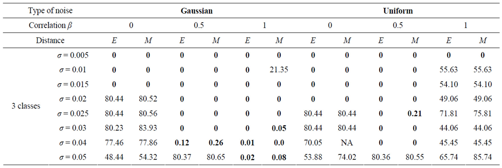 (b)
(b)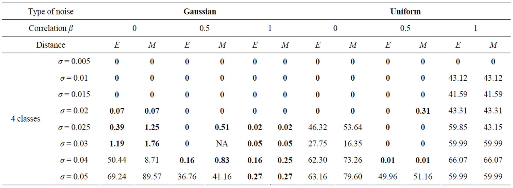 (c)
(c)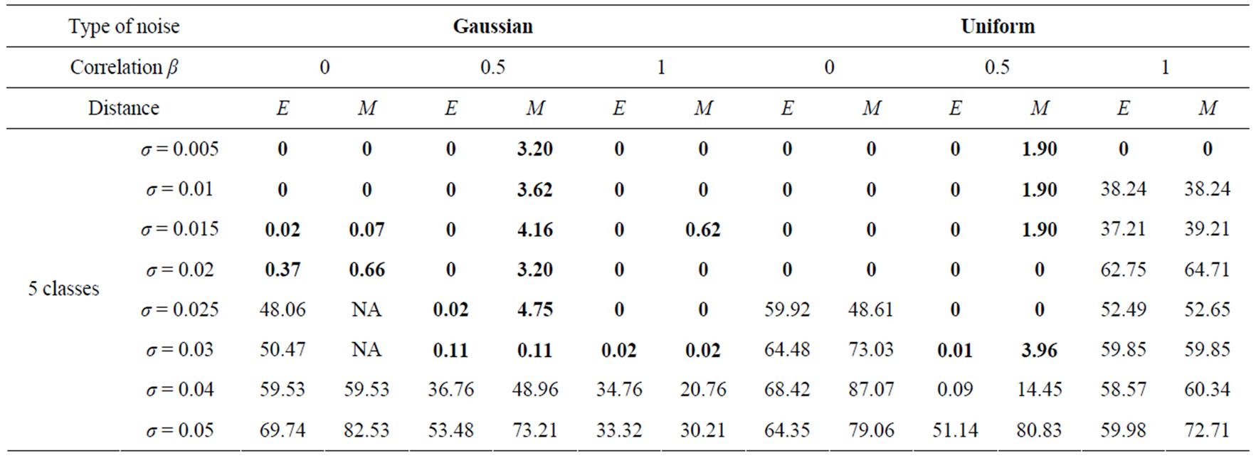 (d)
(d)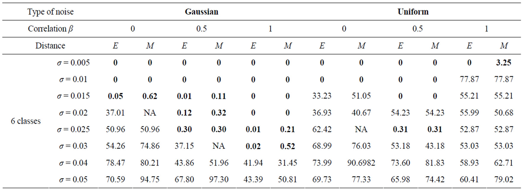 (e)
(e)
Table 3. Segmentation errors in percentage (%) for the probe image of Figure 3, altered with Gaussian or uniform noise. Uncorrelated noise (β = 0), partial correlation, noise (β = 0.5) and totally correlation noise (β = 1). σ is the standard deviation of the noise. The distance used for attributing pixels to different classes is either the Euclidian distance (E) or the Mahalanobis distance (M). The boxes marked NA correspond to cases where the threshold S adjustment does not allow obtaining the desired class number.
robust in Euclidean metric than Mahalanobis metric (Table 3).
The robustness of the segmentation algorithm decreases when the desired number of classes increases. These results come from the fact that the ‘colorimetric’ distance between the two nearest classes decreases when the number on classes increases. Consider ∆, the normalized distance between nearest classes, the segmentation algorithm fails when σ approaches ∆/2.
The histograms peaks are kept separated, even for high noise for a totally correlated noise. However, the segmentation is not very robust to totally correlated Uniform noise because the ‘colorimetric’ variations induced by the noise give rise to new peaks.
6. Conclusions
Image segmentation is an important and sensitive step in image processing through various applications because it affects the interpretation and decision making, which justifies here the study of the influence of noise on the quality of segmentation.
Thus in this article, we presented the performances of our segmentation algorithm in the presence of additive noises. This can be useful in courses offered at the academic level. This article opens the way to the study of non-additive noises, i.e., is multiplicative, see convolutive which may require the use of homomorphic processing. Also an enhancement of the histogram is desirable before segmentation. Certain noises inerrant with the acquisition systems of images such as the speckle noise could be studied. The study of the variation of the fuzzy parameter α in the process of segmentation may be considered because it is likely to promote minimization of error rates of segmentation due to the noise.
7. REFERENCES
- M. Ciuc, “Multicomponent Images Processing: Application to Color Imaging and Radar,” Ph.D. Thesis, University of Bucarest, Roumanie, 2002.
- P. Lambert and L. Macaire, “Filtering and Segmentation: the Specificity of Colour Images,” Proceedings of the First International Conference on Color in Graphics and Image Processing (CGIP), Saint-Etienne, France, 2000, pp. 57-71.
- S. Ouattara, G. L. Loum and A. Clément, “Unsupervised Segmentation Method of Multicomponent Images Based on Fuzzy Connectivity Analysis in Multidimensional Histograms,” Engineering, Vol. 3, No. 3, 2011, pp. 203-214. doi:10.4236/eng.2011.33024
- A. Clément and B. Vigouroux, “A Compact Histogram for the Analysis of Multicomponent Images,” Proceedings of 18th Conference GRETSI on Signal Processing, France, Vol. 1, 2001, pp. 305-307.
- J. Chanussot, A. Clément, B. Vigouroux and J. Chabod, “Lossless Compact Histogram Representation for Multi- Component Images: Application to Histogram Equalization,” Geoscience and Remote Sensing Symposim, (IGARSS), Proceedings of IEEE International, Vol. 6, 2003, pp. 3940- 3942. doi:10.1109/IGARSS.2003.1295321
- S. Ouattara and A. Clement, “Labelling of Compact Multidimensional Histograms for Analysis of Multicomponent Images,” Proceedings of the 21st Conference GRETSI on the Image Processing, Troyes, 2007, pp. 85-88.
- P. Schmid, “Segmentation of Digitized Dermatoscopic Images by Two-Dimensional Color Clustering,” IEEE Transaction on Medical Imaging, Vol. 18, No. 2, 1999, pp. 164-171. doi:10.1109/42.759124
- F. Kurugollu, B. Sankur and A. C. Harmanci, “Color Image Segmentation Using 2-Diomensional Histogram Multitresholding and Fusion,” Proceedings of the First International Conference on Color Graphics and Image Processing, Saint-Etienne, France, 2000, pp. 152-157. doi:10.1016/S0262-8856(01)00052-X
- A. Clément and B. Vigouroux, “Unsupervised Classification of Pixels in Color Images by Hierarchical Analysis of Bi-Dimensional Histograms,” IEEE International Conference on Systems Man and Cybernetics, Hammamet, Tunisia, Vol. 2, 2002, pp. 85-89.
- O. Lezoray, “Unsupervised 2D Multiband Histogram Clustering and Region for Color Image Segmentation,” Proceedings of the 3rd IEEE International Symposium on Signal Processing and Information Technology, 2003, pp. 267-270.
- O. Lezoray and C. Charrier, “Color Image Segmentation Using Morphological Clustering and Fusion with Automatic Scale Selection,” Pattern Recognition Letters, Vol. 30, No. 4, 2009, pp. 397-406. doi:10.1016/j.patrec.2008.11.005
- R. Furferi, “Colour Classification Method for Recycled Melange Fabrics,” Journal of Applied Science, Vol. 1, No. 1, 2011, pp. 236-246. doi:10.3923/jas.2011.236.246
- S. Yamada and K. Murase, “Effectiveness of Flexible Noise Control Image Processing for Digital Portal Images Using Computed Radiography,” British Journal of Radiology, Vol. 78, 2005, pp. 519-527. doi:10.1259/bjr/26039330
- S. H. Lim, “Characterization of Noise in Digital Photographs for Image Processing,” Proceeding in Digital Photography II, IS&T/SPIE Electronic Imaging, vol. 6069, 2008. doi:10.1117/12.655915
- J.-P. Coquerez and S. Philipp, “Image Analysis: Filtering and Segmentation,” Masson, Paris, 1995.
- L. Vinet, “Segmentation and Mapping of Areas of Stereoscopic Pairs of Images,” Ph.D. Thesis, University of Paris IX Dauphine, Paris, 1991.
- M. Borsotti, P. Campadelli and R. Schettini, “Quantitative Evaluation of Color Image Segmentation Results,” Pattern Recognition Letters Vol. 19, No. 8, 1998, pp. 741-747. doi:10.1016/S0167-8655(98)00052-X
- C. Rosenberger, “Adaptative Evaluation of Image Segmentation Results,” Proceeding of 18th International Conference on Pattern Recognition, Vol. 2, 2006, pp. 399-402. doi:10.1109/ICPR.2006.214
- H. Zhang, J. E. Fritts and S. A. Goldman, “Image Segmentation Evaluation: A Survey of Unsupervised Methods,” Computer Vision and Image Understanding, Vol. 110, No. 2, 2008, pp. 260-280. doi:10.1016/j.cviu.2007.08.003